
快速入门
安装
通过 pip 安装:
pip install lifelines
或
通过 conda 安装:
conda install -c conda-forge lifelines
Kaplan-Meier、Nelson-Aalen和参数模型
注意
对于寻找生存分析介绍的读者,建议从生存分析介绍开始。
让我们从导入一些数据开始。我们需要观察个体的持续时间,以及他们是否“死亡”。
from lifelines.datasets import load_waltons
df = load_waltons() # returns a Pandas DataFrame

print(df.head())
"""
    T  E    group
0   6  1  miR-137
1  13  1  miR-137
2  13  1  miR-137
3  13  1  miR-137
4  19  1  miR-137
"""

T = df['T']
E = df['E']
T 是一个持续时间数组,E 是一个布尔或二进制数组,表示是否观察到“死亡”(或者个体可能被审查)。我们将对此拟合一个Kaplan Meier模型,实现为 KaplanMeierFitter:
from lifelines import KaplanMeierFitter
kmf = KaplanMeierFitter()
kmf.fit(T, event_observed=E)  # or, more succinctly, kmf.fit(T, E)
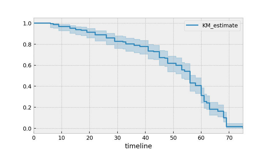
调用fit()方法后,我们可以访问新的属性,如survival_function_和方法,如plot()。后者是Panda内部绘图库的封装。
kmf.survival_function_
kmf.cumulative_density_
kmf.plot_survival_function()
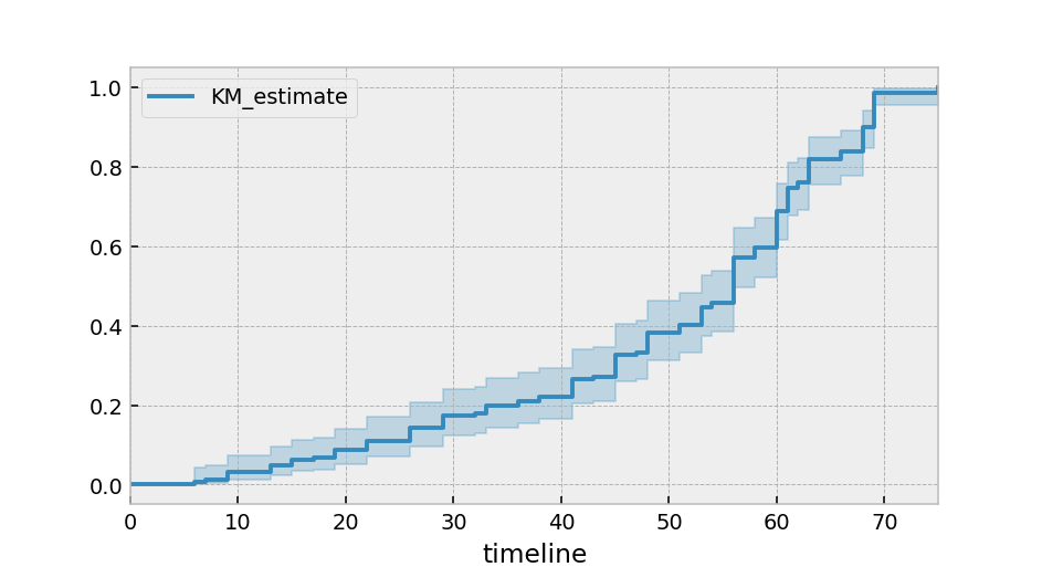
或者,您可以绘制累积密度函数:
kmf.plot_cumulative_density()
通过在fit()中指定timeline关键字参数,我们可以改变上述模型的索引方式:
kmf.fit(T, E, timeline=range(0, 100, 2))

kmf.survival_function_   # index is now the same as range(0, 100, 2)
kmf.confidence_interval_ # index is now the same as range(0, 100, 2)
一个有用的汇总统计是中位生存时间,它表示当50%的人口已经死亡时的时间:
from lifelines.utils import median_survival_times

median_ = kmf.median_survival_time_
median_confidence_interval_ = median_survival_times(kmf.confidence_interval_)
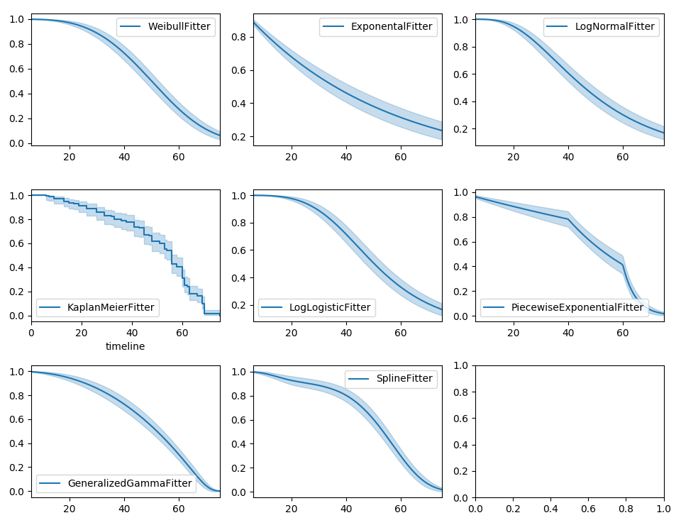
除了Kaplan-Meier估计器,您可能还对参数模型感兴趣。lifelines内置了参数模型。例如,Weibull、Log-Normal、Log-Logistic等。
import matplotlib.pyplot as plt
import numpy as np
from lifelines import *

fig, axes = plt.subplots(3, 3, figsize=(13.5, 7.5))

kmf = KaplanMeierFitter().fit(T, E, label='KaplanMeierFitter')
wbf = WeibullFitter().fit(T, E, label='WeibullFitter')
exf = ExponentialFitter().fit(T, E, label='ExponentialFitter')
lnf = LogNormalFitter().fit(T, E, label='LogNormalFitter')
llf = LogLogisticFitter().fit(T, E, label='LogLogisticFitter')
pwf = PiecewiseExponentialFitter([40, 60]).fit(T, E, label='PiecewiseExponentialFitter')
ggf = GeneralizedGammaFitter().fit(T, E, label='GeneralizedGammaFitter')
sf = SplineFitter(np.percentile(T.loc[E.astype(bool)], [0, 50, 100])).fit(T, E, label='SplineFitter')

wbf.plot_survival_function(ax=axes[0][0])
exf.plot_survival_function(ax=axes[0][1])
lnf.plot_survival_function(ax=axes[0][2])
kmf.plot_survival_function(ax=axes[1][0])
llf.plot_survival_function(ax=axes[1][1])
pwf.plot_survival_function(ax=axes[1][2])
ggf.plot_survival_function(ax=axes[2][0])
sf.plot_survival_function(ax=axes[2][1])
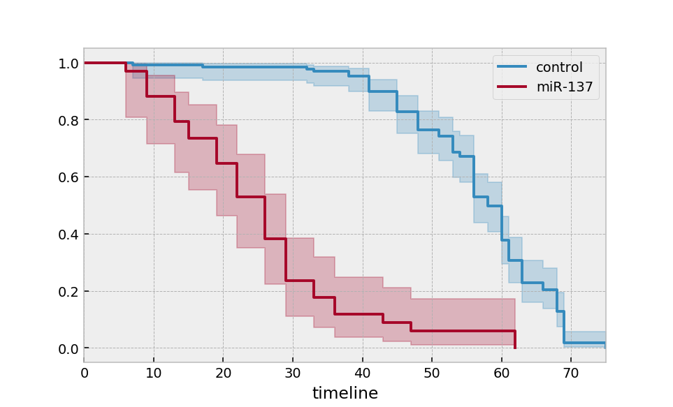
多组
groups = df['group']
ix = (groups == 'miR-137')

kmf.fit(T[~ix], E[~ix], label='control')
ax = kmf.plot_survival_function()

kmf.fit(T[ix], E[ix], label='miR-137')
ax = kmf.plot_survival_function(ax=ax)
或者,对于更多的组和更“pandas风格”的情况:
ax = plt.subplot(111)

kmf = KaplanMeierFitter()

for name, grouped_df in df.groupby('group'):
    kmf.fit(grouped_df["T"], grouped_df["E"], label=name)
    kmf.plot_survival_function(ax=ax)
类似的功能也存在于 NelsonAalenFitter 中:
from lifelines import NelsonAalenFitter
naf = NelsonAalenFitter()
naf.fit(T, event_observed=E)
但是,不是暴露一个survival_function_,而是暴露一个cumulative_hazard_。
注意
类似于Scikit-Learn,所有统计估计的量都会在属性名称后附加一个下划线。
注意
关于估计生存函数和累积风险的更详细文档可在Survival analysis with lifelines中找到。
获取正确格式的数据
通常你会遇到如下所示的数据:
*start_time1*, *end_time1*
*start_time2*, *end_time2*
*start_time3*, None
*start_time4*, *end_time4*
lifelines 有一些实用函数可以将此数据集转换为持续时间和删失向量。最常见的是 lifelines.utils.datetimes_to_durations()。
from lifelines.utils import datetimes_to_durations

# start_times is a vector or list of datetime objects or datetime strings
# end_times is a vector or list of (possibly missing) datetime objects or datetime strings
T, E = datetimes_to_durations(start_times, end_times, freq='h')
也许你有兴趣查看给定一些持续时间和删失向量的生存表。函数 lifelines.utils.survival_table_from_events() 将帮助你实现这一点:
from lifelines.utils import survival_table_from_events

table = survival_table_from_events(T, E)
print(table.head())

"""
          removed  observed  censored  entrance  at_risk
event_at
0               0         0         0       163      163
6               1         1         0         0      163
7               2         1         1         0      162
9               3         3         0         0      160
13              3         3         0         0      157
"""
生存回归
虽然上述的KaplanMeierFitter模型很有用,但它只为我们提供了人群的“平均”视图。通常我们有个体层面的具体数据,我们希望使用这些数据。为此,我们转向生存回归。
注意
更详细的文档和教程可在生存回归中找到。
回归模型的数据集与上述数据集不同。所有数据,包括持续时间、审查指标和协变量,都必须包含在一个Pandas DataFrame中。
from lifelines.datasets import load_regression_dataset
regression_dataset = load_regression_dataset() # a Pandas DataFrame
实例化一个回归模型,并使用fit将模型拟合到数据集。在调用fit时指定了持续时间列和事件列。下面我们使用Cox比例风险模型对我们的回归数据集进行建模,完整文档here。
from lifelines import CoxPHFitter

# Using Cox Proportional Hazards model
cph = CoxPHFitter()
cph.fit(regression_dataset, 'T', event_col='E')
cph.print_summary()

"""
<lifelines.CoxPHFitter: fitted with 200 total observations, 11 right-censored observations>
             duration col = 'T'
                event col = 'E'
      baseline estimation = breslow
   number of observations = 200
number of events observed = 189
   partial log-likelihood = -807.62
         time fit was run = 2020-06-21 12:26:28 UTC

---
       coef  exp(coef)   se(coef)   coef lower 95%   coef upper 95%  exp(coef) lower 95%  exp(coef) upper 95%
var1   0.22       1.25       0.07             0.08             0.37                 1.08                 1.44
var2   0.05       1.05       0.08            -0.11             0.21                 0.89                 1.24
var3   0.22       1.24       0.08             0.07             0.37                 1.07                 1.44

        z      p   -log2(p)
var1 2.99 <0.005       8.49
var2 0.61   0.54       0.89
var3 2.88 <0.005       7.97
---
Concordance = 0.58
Partial AIC = 1621.24
log-likelihood ratio test = 15.54 on 3 df
-log2(p) of ll-ratio test = 9.47
"""

cph.plot()

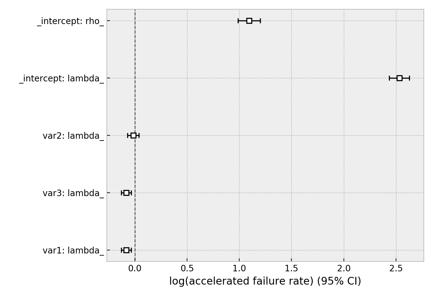
相同的数据集,但使用了威布尔加速失效时间模型。该模型有两个参数(参见文档这里),我们可以选择使用我们的协变量来建模这两个参数,或者只建模其中一个。下面我们只建模尺度参数,lambda_。
from lifelines import WeibullAFTFitter

wft = WeibullAFTFitter()
wft.fit(regression_dataset, 'T', event_col='E')
wft.print_summary()

"""
<lifelines.WeibullAFTFitter: fitted with 200 total observations, 11 right-censored observations>
             duration col = 'T'
                event col = 'E'
   number of observations = 200
number of events observed = 189
           log-likelihood = -504.48
         time fit was run = 2020-06-21 12:27:05 UTC

---
                     coef  exp(coef)   se(coef)   coef lower 95%   coef upper 95%  exp(coef) lower 95%  exp(coef) upper 95%
lambda_ var1        -0.08       0.92       0.02            -0.13            -0.04                 0.88                 0.97
        var2        -0.02       0.98       0.03            -0.07             0.04                 0.93                 1.04
        var3        -0.08       0.92       0.02            -0.13            -0.03                 0.88                 0.97
        Intercept   2.53      12.57       0.05             2.43             2.63                11.41                13.85
rho_    Intercept   1.09       2.98       0.05             0.99             1.20                 2.68                 3.32

                       z      p   -log2(p)
lambda_ var1       -3.45 <0.005      10.78
        var2       -0.56   0.57       0.80
        var3       -3.33 <0.005      10.15
        Intercept 51.12 <0.005        inf
rho_    Intercept 20.12 <0.005     296.66
---
Concordance = 0.58
AIC = 1018.97
log-likelihood ratio test = 19.73 on 3 df
-log2(p) of ll-ratio test = 12.34
"""

wft.plot()
其他AFT模型也可用,请参见这里。另一种回归模型是Aalen的加性模型,它具有随时间变化的危险:
# Using Aalen's Additive model
from lifelines import AalenAdditiveFitter
aaf = AalenAdditiveFitter(fit_intercept=False)
aaf.fit(regression_dataset, 'T', event_col='E')
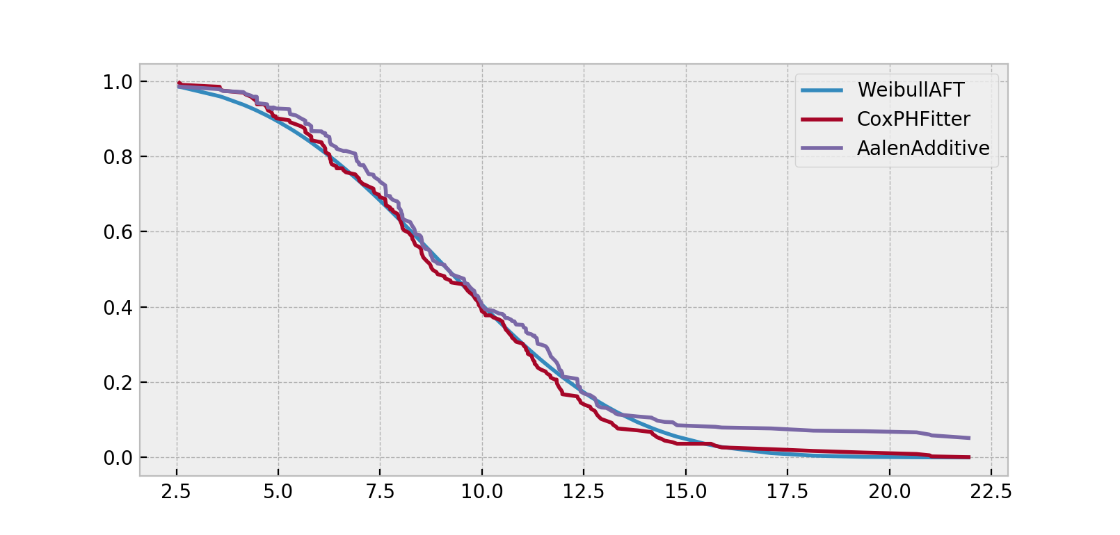
与CoxPHFitter和WeibullAFTFitter一起,拟合后你将可以访问像summary这样的属性和像plot、predict_cumulative_hazards以及predict_survival_function这样的方法。后两种方法需要一个额外的协变量参数:
X = regression_dataset.loc[0]

ax = wft.predict_survival_function(X).rename(columns={0:'WeibullAFT'}).plot()
cph.predict_survival_function(X).rename(columns={0:'CoxPHFitter'}).plot(ax=ax)
aaf.predict_survival_function(X).rename(columns={0:'AalenAdditive'}).plot(ax=ax)
注意
更详细的文档和教程可在生存回归中找到。