
时间滞后的转化率和治愈模型
假设在我们的总体中有一个子总体永远不会经历感兴趣的事件。或者,对于某些受试者来说,事件将在未来非常遥远的时刻发生,几乎等同于无限时间。生存函数不应渐近地趋近于零,而是某个正值。描述这种情况的模型有时被称为治愈模型(即受试者“治愈”了死亡,因此不再易感)或时间滞后转换模型。
在这些类型的问题中使用参数模型存在一个严重的缺陷,而非参数模型则没有这个问题。最常见的参数模型,如Weibull、Log-Normal等,都具有严格递增的累积风险函数,这意味着相应的生存函数将始终收敛到0。
让我们来看一个这个问题的例子。下面我生成了一些数据,这些数据中的个体不会经历该事件,无论我们等待多久。
[1]:
%matplotlib inline
%config InlineBackend.figure_format = 'retina'

from matplotlib import pyplot as plt
import autograd.numpy as np
from autograd.scipy.special import expit, logit
import pandas as pd
plt.style.use('bmh')
[2]:
N = 200
U = np.random.rand(N)
T = -(logit(-np.log(U) / 0.5) - np.random.exponential(2, N) - 6.00) / 0.50

E = ~np.isnan(T)
T[np.isnan(T)] = 50
[5]:
from lifelines import KaplanMeierFitter
kmf = KaplanMeierFitter().fit(T, E)
kmf.plot(figsize=(8,4))
plt.ylim(0, 1);
plt.title("Survival function estimated by KaplanMeier")
[5]:
Text(0.5, 1.0, 'Survival function estimated by KaplanMeier')

应该清楚的是,在0.6左右有一个渐近线。非参数模型总是会显示这一点。如果这是真的,那么累积风险函数也应该有一个水平渐近线。让我们使用Nelson-Aalen模型来看看这一点。
[6]:
from lifelines import NelsonAalenFitter

naf = NelsonAalenFitter().fit(T, E)
naf.plot(figsize=(8,4))
plt.title("Cumulative hazard estimated by NelsonAalen")
[6]:
Text(0.5, 1.0, 'Cumulative hazard estimated by NelsonAalen')

然而,当我们尝试使用参数模型时,我们会发现它的外推效果并不理想。让我们使用灵活的双参数LogLogisticFitter模型。
[11]:
from lifelines import LogLogisticFitter

fig, ax = plt.subplots(nrows=1, ncols=2, figsize=(12, 4))

t = np.linspace(0, 40)
llf = LogLogisticFitter().fit(T, E, timeline=t)

t = np.linspace(0, 100)
llf = LogLogisticFitter().fit(T, E, timeline=t)

llf.plot_survival_function(ax=ax[0])
kmf.plot(ax=ax[0])

llf.plot_cumulative_hazard(ax=ax[1])
naf.plot(ax=ax[1])
[11]:
<AxesSubplot:xlabel='timeline'>

LogLogistic模型不仅在捕捉渐近线方面表现不佳,而且在中间值方面也是如此。如果我们进一步扩展生存函数,我们会发现它最终接近于0。
自定义参数模型以处理渐近线
专注于建模累积风险函数,我们想要的是一个增加到某个极限然后逐渐趋于渐近线的函数。我们可以长时间深入思考这些(我确实这样做了),但有一类函数具有我们非常熟悉的这种特性:累积分布函数!根据它们的性质,它们将渐近地接近1。而且,它们在SciPy和autograd库中很容易获得。因此,我们的累积风险函数的新模型是:
其中 \(c\) 是(未知的)水平渐近线,\(\theta\) 是 CDF \(F\) 的(未知)参数向量。
我们可以使用ParametricUnivariateFitter创建一个自定义的累积风险模型(有关如何创建自定义模型的教程,请参见这里)。让我们选择正态CDF作为我们的模型。
记住我们必须使用autograd的导入,即from autograd.scipy.stats import norm。
[13]:
from autograd.scipy.stats import norm
from lifelines.fitters import ParametricUnivariateFitter


class UpperAsymptoteFitter(ParametricUnivariateFitter):

    _fitted_parameter_names = ["c_", "mu_", "sigma_"]

    _bounds = ((0, None), (None, None), (0, None))

    def _cumulative_hazard(self, params, times):
        c, mu, sigma = params
        return c * norm.cdf((times - mu) / sigma, loc=0, scale=1)
[14]:
uaf = UpperAsymptoteFitter().fit(T, E)
uaf.print_summary(3)
uaf.plot(figsize=(8,4))
| model | lifelines.UpperAsymptoteFitter |
|---|---|
| number of observations | 200 |
| number of events observed | 83 |
| log-likelihood | -382.304 |
| hypothesis | c_ != 1, mu_ != 0, sigma_ != 1 |
| coef | se(coef) | coef lower 95% | coef upper 95% | z | p | -log2(p) | |
|---|---|---|---|---|---|---|---|
| c_ | 0.539 | 0.060 | 0.422 | 0.657 | -7.701 | <0.0005 | 46.069 |
| mu_ | 17.397 | 0.527 | 16.364 | 18.429 | 33.015 | <0.0005 | 791.632 |
| sigma_ | 4.746 | 0.369 | 4.022 | 5.470 | 10.142 | <0.0005 | 77.880 |
| AIC | 770.608 |
|---|
[14]:
<AxesSubplot:>
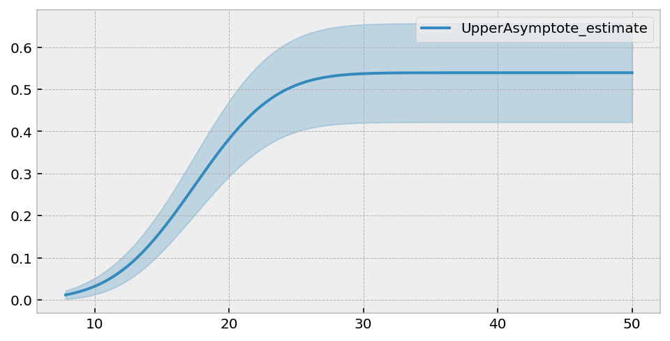
我们得到了一个美丽的渐近累积风险。汇总表表明,\(c\)的最佳值是0.586。这可以通过\(\exp(-0.586) \approx 0.56\)转化为生存函数的渐近线。
让我们将这个拟合与非参数模型进行比较。
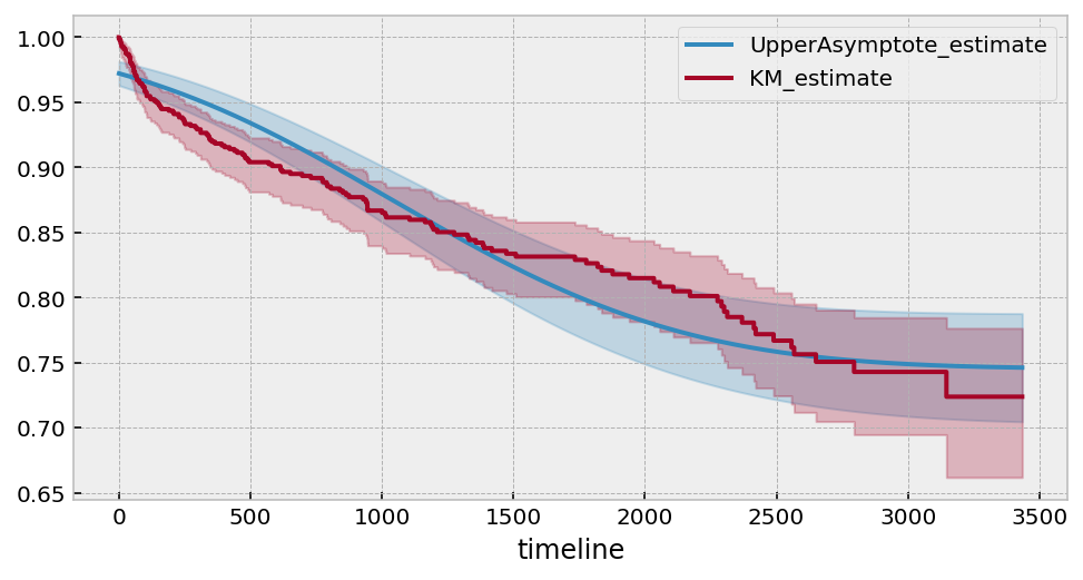
[15]:
fig, ax = plt.subplots(nrows=2, ncols=2, figsize=(10, 6))

t = np.linspace(0, 40)
uaf = UpperAsymptoteFitter().fit(T, E, timeline=t)

uaf.plot_survival_function(ax=ax[0][0])
kmf.plot(ax=ax[0][0])

uaf.plot_cumulative_hazard(ax=ax[0][1])
naf.plot(ax=ax[0][1])

t = np.linspace(0, 100)
uaf = UpperAsymptoteFitter().fit(T, E, timeline=t)
uaf.plot_survival_function(ax=ax[1][0])
kmf.survival_function_.plot(ax=ax[1][0])

uaf.plot_cumulative_hazard(ax=ax[1][1])
naf.plot(ax=ax[1][1])
[15]:
<AxesSubplot:xlabel='timeline'>

我没想到会有这么好的拟合效果。但事实就是如此。这是一些人工数据,但让我们在一些真实数据上试试这个技术。
[18]:
from lifelines.datasets import load_leukemia, load_kidney_transplant

T, E = load_leukemia()['t'], load_leukemia()['status']
uaf.fit(T, E)
ax = uaf.plot_survival_function(figsize=(8,4))
uaf.print_summary()

kmf.fit(T, E).plot(ax=ax, ci_show=False)
print("---")
print("Estimated lower bound: {:.2f} ({:.2f}, {:.2f})".format(
        np.exp(-uaf.summary.loc['c_', 'coef']),
        np.exp(-uaf.summary.loc['c_', 'coef upper 95%']),
        np.exp(-uaf.summary.loc['c_', 'coef upper 95%']),
    )
)
| model | lifelines.UpperAsymptoteFitter |
|---|---|
| number of observations | 42 |
| number of events observed | 30 |
| log-likelihood | -118.60 |
| hypothesis | c_ != 1, mu_ != 0, sigma_ != 1 |
| coef | se(coef) | coef lower 95% | coef upper 95% | z | p | -log2(p) | |
|---|---|---|---|---|---|---|---|
| c_ | 1.63 | 0.36 | 0.94 | 2.33 | 1.78 | 0.07 | 3.75 |
| mu_ | 13.44 | 1.73 | 10.06 | 16.82 | 7.79 | <0.005 | 47.07 |
| sigma_ | 7.03 | 1.07 | 4.94 | 9.12 | 5.65 | <0.005 | 25.91 |
| AIC | 243.20 |
|---|
---
Estimated lower bound: 0.20 (0.10, 0.10)

因此,我们可能预计大约20%的人在这个群体中不会发生该事件(但也要注意较大的置信区间界限!)
[21]:
# Another, less obvious, dataset.

T, E = load_kidney_transplant()['time'], load_kidney_transplant()['death']
uaf.fit(T, E)
ax = uaf.plot_survival_function(figsize=(8,4))
uaf.print_summary()

kmf.fit(T, E).plot(ax=ax)
print("---")
print("Estimated lower bound: {:.2f} ({:.2f}, {:.2f})".format(
        np.exp(-uaf.summary.loc['c_', 'coef']),
        np.exp(-uaf.summary.loc['c_', 'coef upper 95%']),
        np.exp(-uaf.summary.loc['c_', 'coef lower 95%']),
    )
)
| model | lifelines.UpperAsymptoteFitter |
|---|---|
| number of observations | 863 |
| number of events observed | 140 |
| log-likelihood | -1458.88 |
| hypothesis | c_ != 1, mu_ != 0, sigma_ != 1 |
| coef | se(coef) | coef lower 95% | coef upper 95% | z | p | -log2(p) | |
|---|---|---|---|---|---|---|---|
| c_ | 0.29 | 0.03 | 0.24 | 0.35 | -24.37 | <0.005 | 433.49 |
| mu_ | 1139.88 | 101.60 | 940.75 | 1339.01 | 11.22 | <0.005 | 94.62 |
| sigma_ | 872.59 | 66.31 | 742.62 | 1002.56 | 13.14 | <0.005 | 128.67 |
| AIC | 2923.76 |
|---|
---
Estimated lower bound: 0.75 (0.70, 0.79)
使用替代函数形式
一个更简单的模型可能看起来像 \(c \left(1 - \frac{1}{\lambda t + 1}\right)\),然而这个模型无法处理任何“拐点”,就像我们的人工数据集上面那样。然而,它在这个肺部数据集上表现良好。
对于所有参数模型,一个重要的特征是能够外推到未预见的时间。
[22]:
from autograd.scipy.stats import norm
from lifelines.fitters import ParametricUnivariateFitter

class SimpleUpperAsymptoteFitter(ParametricUnivariateFitter):

    _fitted_parameter_names = ["c_", "lambda_"]

    _bounds = ((0, None), (0, None))

    def _cumulative_hazard(self, params, times):
        c, lambda_ = params
        return c * (1 -  1 /(lambda_ * times + 1))
[23]:
# Another, less obvious, dataset.

saf = SimpleUpperAsymptoteFitter().fit(T, E, timeline=np.arange(1, 10000))
ax = saf.plot_survival_function(figsize=(8,4))
saf.print_summary(4)

kmf.fit(T, E).plot(ax=ax)
print("---")
print("Estimated lower bound: {:.2f} ({:.2f}, {:.2f})".format(
        np.exp(-saf.summary.loc['c_', 'coef']),
        np.exp(-saf.summary.loc['c_', 'coef upper 95%']),
        np.exp(-saf.summary.loc['c_', 'coef lower 95%']),
    )
)
| model | lifelines.SimpleUpperAsymptoteFitter |
|---|---|
| number of observations | 863 |
| number of events observed | 140 |
| log-likelihood | -1392.1610 |
| hypothesis | c_ != 1, lambda_ != 1 |
| coef | se(coef) | coef lower 95% | coef upper 95% | z | p | -log2(p) | |
|---|---|---|---|---|---|---|---|
| c_ | 0.4252 | 0.0717 | 0.2847 | 0.5658 | -8.0151 | <5e-05 | 49.6912 |
| lambda_ | 0.0006 | 0.0002 | 0.0003 | 0.0009 | -5982.3551 | <5e-05 | inf |
| AIC | 2788.3221 |
|---|
---
Estimated lower bound: 0.65 (0.57, 0.75)

概率治愈模型
上述模型在拟合数据方面表现良好,但它们对生存模型的常见解释较少。能够使用常见的生存模型并且具有一些“治愈”成分将会很好。让我们假设对于将经历感兴趣事件的个体,他们的生存分布是威布尔分布,表示为\(S_W(t)\)。对于在人群中随机选择的个体,他们的生存曲线\(S(t)\)是:
尽管它以一种非常规的形式存在,我们仍然可以确定累积风险(这是生存函数的负对数):
[24]:
from autograd import numpy as np
from lifelines.fitters import ParametricUnivariateFitter

class CureFitter(ParametricUnivariateFitter):

    _fitted_parameter_names = ["p_", "lambda_", "rho_"]

    _bounds = ((0, 1), (0, None), (0, None))

    def _cumulative_hazard(self, params, T):
        p, lambda_, rho_ = params
        sf = np.exp(-(T / lambda_) ** rho_)
        return -np.log(p + (1-p) * sf)
[25]:
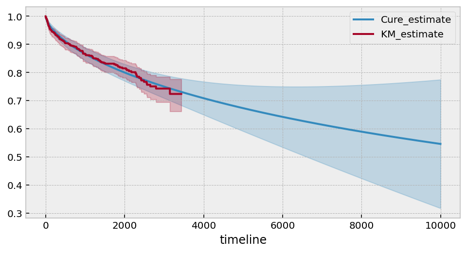
cure_model = CureFitter().fit(T, E, timeline=np.arange(1, 10000))
ax = cure_model.plot_survival_function(figsize=(8,4))
cure_model.print_summary(4)

kmf.fit(T, E).plot(ax=ax)
print("---")
print("Estimated lower bound: {:.2f} ({:.2f}, {:.2f})".format(
        cure_model.summary.loc['p_', 'coef'],
        cure_model.summary.loc['p_', 'coef upper 95%'],
        cure_model.summary.loc['p_', 'coef lower 95%'],
    )
)
| model | lifelines.CureFitter |
|---|---|
| number of observations | 863 |
| number of events observed | 140 |
| log-likelihood | -1385.1617 |
| hypothesis | p_ != 0.5, lambda_ != 1, rho_ != 1 |
| coef | se(coef) | coef lower 95% | coef upper 95% | z | p | -log2(p) | |
|---|---|---|---|---|---|---|---|
| p_ | 0.1006 | 1.3053 | -2.4577 | 2.6590 | -0.3059 | 0.7596 | 0.3966 |
| lambda_ | 17393.6107 | 48891.6027 | -78432.1698 | 113219.3911 | 0.3557 | 0.7220 | 0.4699 |
| rho_ | 0.6382 | 0.0791 | 0.4831 | 0.7932 | -4.5739 | <5e-05 | 17.6725 |
| AIC | 2776.3234 |
|---|
---
Estimated lower bound: 0.10 (2.66, -2.46)
在这种模型下,它表明只有约10%的受试者被治愈(然而,\(p\)参数的估计值存在很大差异)。