
分段指数模型和创建自定义模型
如果我们回忆起我们的三个数学“生物”以及它们之间的关系,这一部分将会更容易理解。首先是生存函数,\(S(t)\),它表示活过某个时间\(t\)的概率。接下来是始终非负且非递减的累积风险函数,\(H(t)\)。它与\(S(t)\)的关系是:
最后,风险函数\(h(t)\)是累积风险的导数:
它与生存函数有直接的关系:
请注意,这三个中的任何一个都绝对定义了其他两个。某些情况下,定义其中一个比定义其他两个更容易。例如,在Cox模型中,最容易处理的是风险\(h(t)\)。在本节关于参数单变量模型的部分中,最容易处理的是累积风险。这是因为数学中的不对称性:导数比积分更容易计算。因此,如果我们定义了累积风险,那么风险函数和生存函数都比我们定义风险并询问其他两个问题时要容易得多。
首先,让我们回顾一些更简单的参数模型。
指数模型
回想一下,指数模型具有恒定的风险,即:
这意味着累积风险\(H(t)\)有一个非常简单的形式:\(H(t) = \frac{t}{\lambda}\)。下面我们将这个模型拟合到一些生存数据上。
[1]:
%matplotlib inline
%config InlineBackend.figure_format = 'retina'

from matplotlib import pyplot as plt
import numpy as np
import pandas as pd

from lifelines.datasets import load_waltons
waltons = load_waltons()
T, E = waltons['T'], waltons['E']
[2]:
from lifelines import ExponentialFitter

fig, ax = plt.subplots(nrows=1, ncols=2, figsize=(10, 4))

epf = ExponentialFitter().fit(T, E)
epf.plot_hazard(ax=ax[0])
epf.plot_cumulative_hazard(ax=ax[1])

ax[0].set_title("hazard"); ax[1].set_title("cumulative_hazard")

epf.print_summary(3)
| model | lifelines.ExponentialFitter |
|---|---|
| number of observations | 163 |
| number of events observed | 156 |
| log-likelihood | -771.913 |
| hypothesis | lambda_ != 1 |
| coef | se(coef) | coef lower 95% | coef upper 95% | z | p | -log2(p) | |
|---|---|---|---|---|---|---|---|
| lambda_ | 51.840 | 4.151 | 43.705 | 59.975 | 12.249 | <0.0005 | 112.180 |
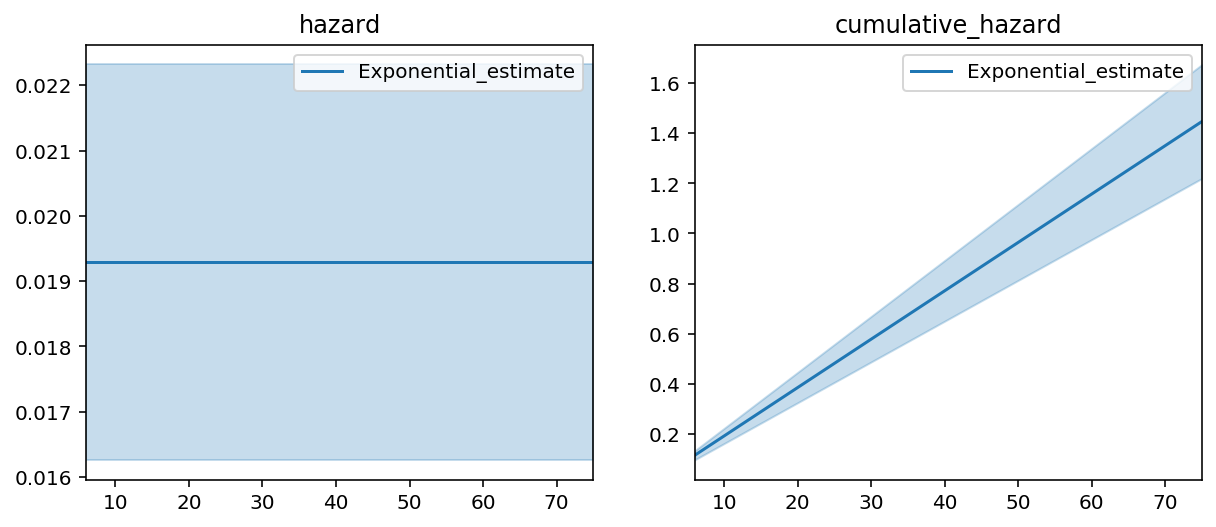
这个模型在拟合我们的数据方面表现不佳。如果我拟合一个非参数模型,比如Nelson-Aalen模型,到这个数据上,指数分布的拟合不足非常明显。
[3]:
from lifelines import NelsonAalenFitter

ax = epf.plot(figsize=(8,5))

naf = NelsonAalenFitter().fit(T, E)
ax = naf.plot(ax=ax)
plt.legend()
[3]:
<matplotlib.legend.Legend at 0x126f5c630>
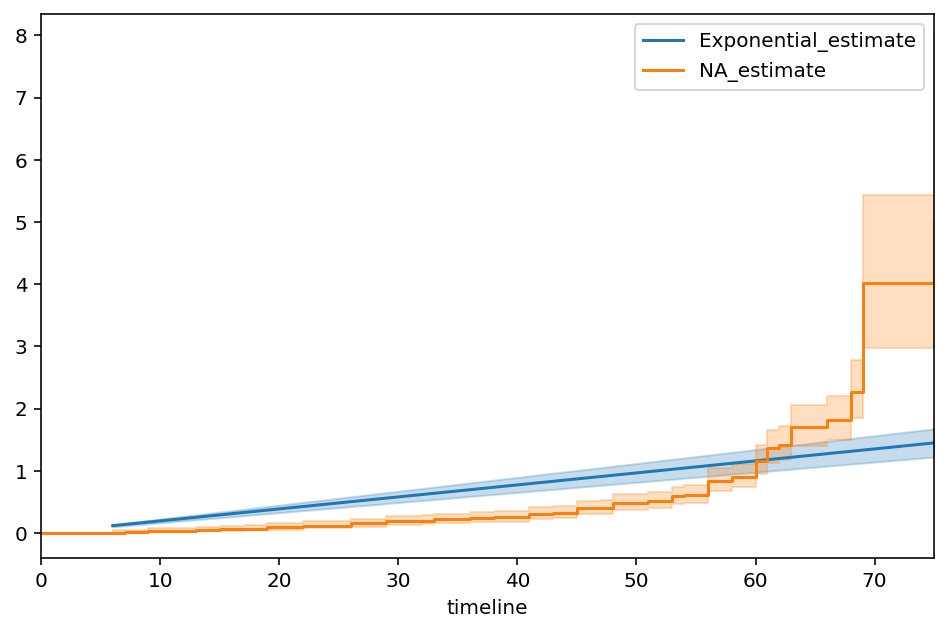
应该清楚的是,单参数模型只是在整个时间段内对风险进行平均。然而,实际上,真实的风险率表现出一些复杂的非线性行为。
分段指数模型
如果我们可以将模型分解为不同的时间段,并为每个时间段拟合一个指数模型,会怎样?例如,我们将风险定义为:
这个模型应该足够灵活,以更好地适应我们的数据集。
累积风险稍微复杂一些,但并不是太复杂,仍然可以在Python中定义。在lifelines中,单变量模型的构建使得人们只需定义感兴趣的参数的累积风险模型,而拟合、创建置信区间、绘图等所有繁重的工作都由系统处理。
例如,lifelines 已经实现了 PiecewiseExponentialFitter 模型。在内部,代码是一个定义累积风险的单一函数。用户指定他们认为的“断点”位置,lifelines 估计最佳的 \(\lambda_i\)。
[4]:
from lifelines import PiecewiseExponentialFitter

# looking at the above plot, I think there may be breaks at t=40 and t=60.
pf = PiecewiseExponentialFitter(breakpoints=[40, 60]).fit(T, E)

fig, axs = plt.subplots(nrows=1, ncols=2, figsize=(10, 4))

ax = pf.plot(ax=axs[1])
pf.plot_hazard(ax=axs[0])

ax = naf.plot(ax=ax, ci_show=False)
axs[0].set_title("hazard"); axs[1].set_title("cumulative_hazard")

pf.print_summary(3)
| model | lifelines.PiecewiseExponentialFitter |
|---|---|
| number of observations | 163 |
| number of events observed | 156 |
| log-likelihood | -647.118 |
| hypothesis | lambda_0_ != 1, lambda_1_ != 1, lambda_2_ != 1 |
| coef | se(coef) | coef lower 95% | coef upper 95% | z | p | -log2(p) | |
|---|---|---|---|---|---|---|---|
| lambda_0_ | 162.989 | 27.144 | 109.787 | 216.191 | 5.968 | <0.0005 | 28.630 |
| lambda_1_ | 31.366 | 4.043 | 23.442 | 39.290 | 7.511 | <0.0005 | 43.957 |
| lambda_2_ | 4.686 | 0.624 | 3.462 | 5.910 | 5.902 | <0.0005 | 28.055 |
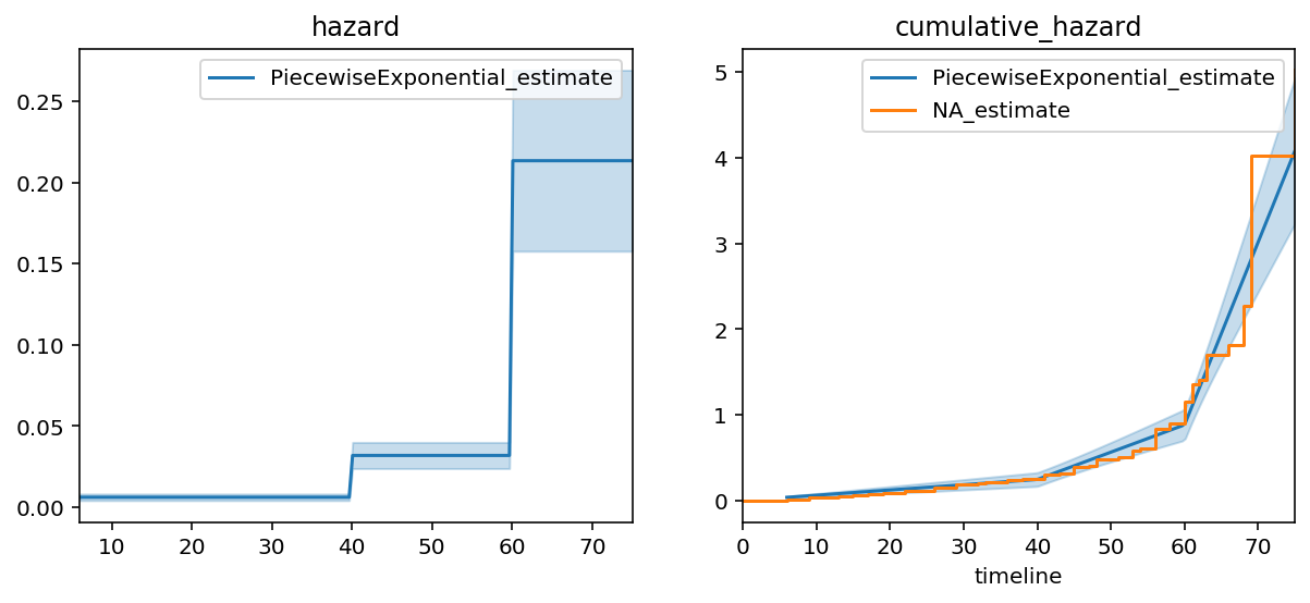
我们可以看到这个模型的拟合效果要好得多。拟合的定量测量是比较指数模型和分段指数模型之间的对数似然(越高越好)。对数似然分别从-772增加到-647。我们可以继续添加更多的断点,但这最终会导致对数据的过拟合。
lifelines中的单变量模型
我提到过PiecewiseExponentialFitter仅使用其累积风险函数实现。这不是谎言。lifelines对于单变量拟合器有非常通用的语义。例如,这是整个ExponentialFitter的实现方式:
class ExponentialFitter(ParametricUnivariateFitter):

    _fitted_parameter_names = ["lambda_"]

    def _cumulative_hazard(self, params, times):
        lambda_ = params[0]
        return times / lambda_
我们只需要指定累积风险函数,因为累积风险函数与生存函数和风险率之间存在1:1:1的关系。从那里开始,lifelines 会处理其余的部分。
定义我们自己的生存模型
为了展示lifelines单变量模型的灵活性,我们将创建一个全新的、前所未见的生存模型。观察Nelson-Aalen拟合,累积危险看起来在\(t=80\)处可能有一个渐近线。这可能对应于受试者生命的绝对上限。让我们从那个函数形式开始。
我们使用下标 \(1\) 是因为我们将研究其他模型。在 lifelines 单变量模型中,这由以下代码定义。
重要: 为了计算导数,你必须使用从autograd库导入的numpy。这是对原始numpy的一个轻量级封装。请注意下面的import autograd.numpy as np。
[5]:
from lifelines.fitters import ParametricUnivariateFitter

import autograd.numpy as np

class InverseTimeHazardFitter(ParametricUnivariateFitter):

    # we tell the model what we want the names of the unknown parameters to be
    _fitted_parameter_names = ['alpha_']


    # this is the only function we need to define. It always takes two arguments:
    #   params: an iterable that unpacks the parameters you'll need in the order of _fitted_parameter_names
    #   times: a vector of times that will be passed in.
    def _cumulative_hazard(self, params, times):
        alpha = params[0]
        return alpha /(80 - times)
[6]:
itf = InverseTimeHazardFitter()
itf.fit(T, E)
itf.print_summary()

ax = itf.plot(figsize=(8,5))
ax = naf.plot(ax=ax, ci_show=False)
plt.legend()
| model | lifelines.InverseTimeHazardFitter |
|---|---|
| number of observations | 163 |
| number of events observed | 156 |
| log-likelihood | -697.84 |
| hypothesis | alpha_ != 1 |
| coef | se(coef) | coef lower 95% | coef upper 95% | z | p | -log2(p) | |
|---|---|---|---|---|---|---|---|
| alpha_ | 21.51 | 1.72 | 18.13 | 24.88 | 11.91 | <0.005 | 106.22 |
[6]:
<matplotlib.legend.Legend at 0x127597198>

模型对数据的最佳拟合是:
我们选择80作为渐近线可能是错误的,所以让我们允许渐近线成为另一个参数:
如果我们以这种方式定义模型,我们需要为\(\beta\)可以取的值添加一个界限。显然,它不能小于或等于观察到的最大持续时间。通常,累积风险必须是正数且非递减的。否则,模型拟合将遇到收敛问题。
[7]:
class TwoParamInverseTimeHazardFitter(ParametricUnivariateFitter):

    _fitted_parameter_names = ['alpha_', 'beta_']

    # Sequence of (min, max) pairs for each element in x. None is used to specify no bound
    _bounds = [(0, None), (75.0001, None)]

    def _cumulative_hazard(self, params, times):
        alpha, beta = params
        return alpha / (beta - times)
[8]:
two_f = TwoParamInverseTimeHazardFitter()
two_f.fit(T, E)
two_f.print_summary()

ax = itf.plot(ci_show=False, figsize=(8,5))
ax = naf.plot(ax=ax, ci_show=False)
two_f.plot(ax=ax)
plt.legend()
| model | lifelines.TwoParamInverseTimeHazardFitter |
|---|---|
| number of observations | 163 |
| number of events observed | 156 |
| log-likelihood | -685.57 |
| hypothesis | alpha_ != 1, beta_ != 76.0001 |
| coef | se(coef) | coef lower 95% | coef upper 95% | z | p | -log2(p) | |
|---|---|---|---|---|---|---|---|
| alpha_ | 16.50 | 1.51 | 13.55 | 19.46 | 10.28 | <0.005 | 79.98 |
| beta_ | 76.55 | 0.38 | 75.80 | 77.30 | 1.44 | 0.15 | 2.73 |
[8]:
<matplotlib.legend.Legend at 0x127247080>
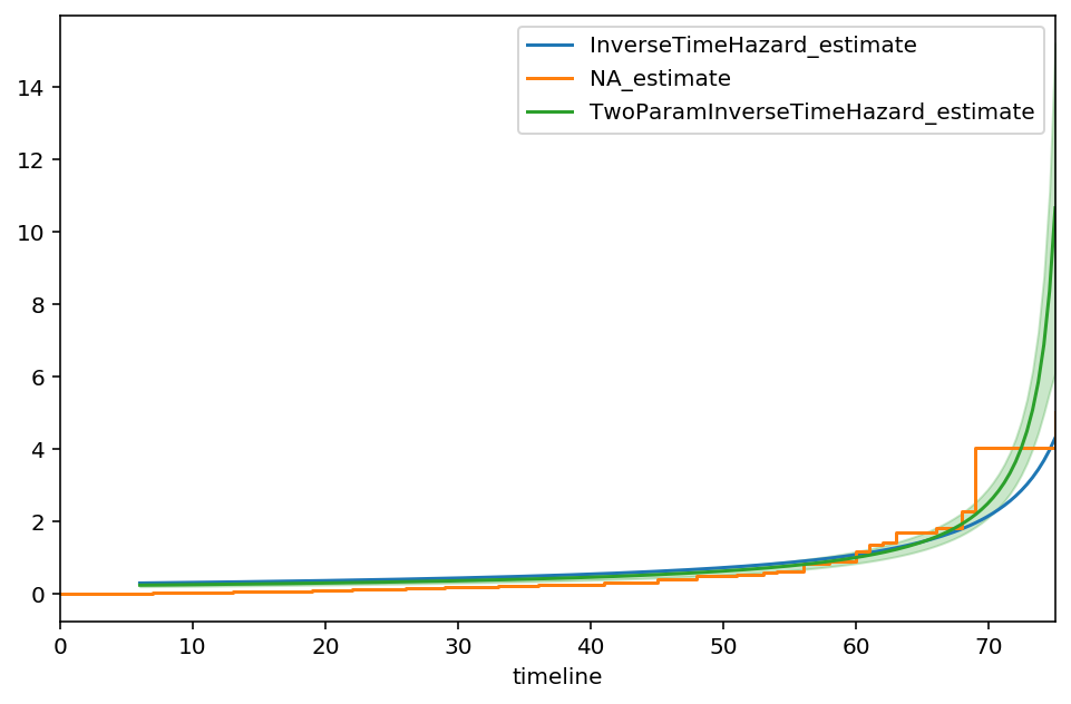
从输出中,我们看到76.55的值是建议的渐近线,即:
曲线似乎也更符合Nelson-Aalen模型。让我们尝试一个额外的参数,\(\gamma\),某种衰减的度量。
[9]:
from lifelines.fitters import ParametricUnivariateFitter

class ThreeParamInverseTimeHazardFitter(ParametricUnivariateFitter):

    _fitted_parameter_names = ['alpha_', 'beta_', 'gamma_']
    _bounds = [(0, None), (75.0001, None), (0, None)]

    # this is the only function we need to define. It always takes two arguments:
    #   params: an iterable that unpacks the parameters you'll need in the order of _fitted_parameter_names
    #   times: a numpy vector of times that will be passed in by the optimizer
    def _cumulative_hazard(self, params, times):
        a, b, c = params
        return a / (b - times) ** c
[10]:
three_f = ThreeParamInverseTimeHazardFitter()
three_f.fit(T, E)
three_f.print_summary()

ax = itf.plot(ci_show=False, figsize=(8,5))
ax = naf.plot(ax=ax, ci_show=False)
ax = two_f.plot(ax=ax, ci_show=False)
ax = three_f.plot(ax=ax)
plt.legend()
| model | lifelines.ThreeParamInverseTimeHazardFitter |
|---|---|
| number of observations | 163 |
| number of events observed | 156 |
| log-likelihood | -649.38 |
| hypothesis | alpha_ != 1, beta_ != 76.0001, gamma_ != 1 |
| coef | se(coef) | coef lower 95% | coef upper 95% | z | p | -log2(p) | |
|---|---|---|---|---|---|---|---|
| alpha_ | 1588776.28 | 3775137.44 | -5810357.13 | 8987909.70 | 0.42 | 0.67 | 0.57 |
| beta_ | 100.88 | 5.88 | 89.35 | 112.41 | 4.23 | <0.005 | 15.38 |
| gamma_ | 3.83 | 0.50 | 2.85 | 4.81 | 5.64 | <0.005 | 25.82 |
[10]:
<matplotlib.legend.Legend at 0x126aa6f60>

我们的新渐近线位于\(t\approx 100, \text{c.i.}=(87, 112)\)。该模型似乎比之前的模型更好地拟合了早期时间,然而我们的\(\alpha\)参数现在有更多的不确定性。继续添加参数是不可取的,因为我们会过度拟合数据。
为什么要拟合参数模型呢?退一步说,我们正在拟合参数模型并将其与非参数的Nelson-Aalen模型进行比较。为什么不总是使用Nelson-Aalen模型呢?
有时我们有科学动机使用参数模型。也就是说,利用领域知识,我们可能知道系统有一个参数模型,并且我们希望拟合该模型。
在参数模型中,我们从所有观察中借用信息来确定最佳参数。为了更清楚地说明这一点,想象一下取一个观察值并大幅改变其值。拟合参数也会随之改变。另一方面,想象一下对非参数模型做同样的事情。在这种情况下,只有局部生存函数或风险函数会发生变化。因为参数模型可以从所有观察中借用信息,并且未知数比非参数模型少得多,所以参数模型被认为具有更高的统计效率。
外推:非参数模型不容易扩展到观察数据之外的值。另一方面,参数模型在这方面没有问题。然而,在观察值之外进行外推是非常危险的行为。
[11]:
fig, axs = plt.subplots(3, figsize=(7, 8), sharex=True)

new_timeline = np.arange(0, 85)

three_f = ThreeParamInverseTimeHazardFitter().fit(T, E, timeline=new_timeline)

three_f.plot_hazard(label='hazard', ax=axs[0]).legend()
three_f.plot_cumulative_hazard(label='cumulative hazard',  ax=axs[1]).legend()
three_f.plot_survival_function(label='survival function',  ax=axs[2]).legend()

fig.subplots_adjust(hspace=0)
# Hide x labels and tick labels for all but bottom plot.
for ax in axs:
    ax.label_outer()
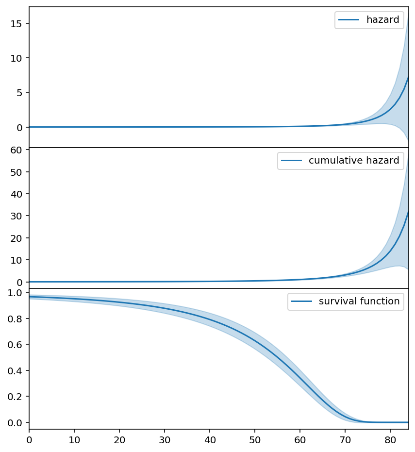
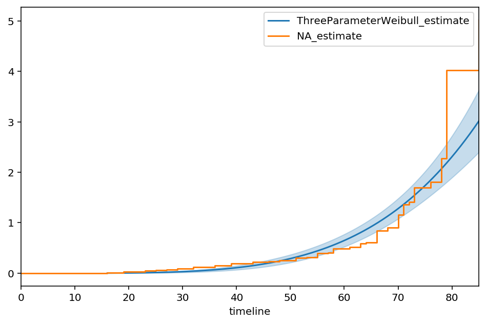
三参数威布尔分布
我们可以轻松地扩展内置的Weibull模型(lifelines.WeibullFitter)以包含一个新的位置参数:
(当\(\theta = 0\)时,这又回到了2参数的情况)。在lifelines自定义模型中,这看起来像:
[90]:
import autograd.numpy as np
from autograd.scipy.stats import norm

# I'm shifting this to exaggerate the effect
T_ = T + 10

class ThreeParameterWeibullFitter(ParametricUnivariateFitter):

    _fitted_parameter_names = ["lambda_", "rho_", "theta_"]
    _bounds = [(0, None), (0, None), (0, T.min()-0.001)]

    def _cumulative_hazard(self, params, times):
        lambda_, rho_, theta_ = params
        return ((times - theta_) / lambda_) ** rho_
[92]:
tpw = ThreeParameterWeibullFitter()
tpw.fit(T_, E)
tpw.print_summary()
ax = tpw.plot_cumulative_hazard(figsize=(8,5))
ax = NelsonAalenFitter().fit(T_, E).plot(ax=ax, ci_show=False)
| model | lifelines.ThreeParameterWeibullFitter |
|---|---|
| number of observations | 163 |
| number of events observed | 156 |
| log-likelihood | -665.49 |
| hypothesis | lambda_ != 1, rho_ != 1, theta_ != 2.9995 |
| coef | se(coef) | coef lower 95% | coef upper 95% | z | p | -log2(p) | |
|---|---|---|---|---|---|---|---|
| lambda_ | 66.21 | 6.24 | 53.98 | 78.44 | 10.45 | <0.005 | 82.52 |
| rho_ | 4.42 | 0.62 | 3.20 | 5.64 | 5.49 | <0.005 | 24.53 |
| theta_ | 0.00 | 5.92 | -11.59 | 11.59 | -0.51 | 0.61 | 0.71 |
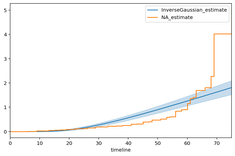
逆高斯分布
逆高斯分布是生存分析中另一个流行的模型。与其他模型不同,其危险率不会渐近收敛到0,从而允许生存的长尾。让我们使用Wikipedia中的相同参数化来建模。
[93]:
from autograd.scipy.stats import norm


class InverseGaussianFitter(ParametricUnivariateFitter):
    _fitted_parameter_names = ['lambda_', 'mu_']

    def _cumulative_density(self, params, times):
        mu_, lambda_ = params
        v = norm.cdf(np.sqrt(lambda_ / times) * (times / mu_ - 1), loc=0, scale=1) + \
               np.exp(2 * lambda_ / mu_) * norm.cdf(-np.sqrt(lambda_ / times) * (times / mu_ + 1), loc=0, scale=1)
        return v

    def _cumulative_hazard(self, params, times):
        return -np.log(1-np.clip(self._cumulative_density(params, times), 1e-15, 1-1e-15))
[94]:
igf = InverseGaussianFitter()
igf.fit(T, E)
igf.print_summary()
ax = igf.plot_cumulative_hazard(figsize=(8,5))
ax = NelsonAalenFitter().fit(T, E).plot(ax=ax, ci_show=False)
| model | lifelines.InverseGaussianFitter |
|---|---|
| number of observations | 163 |
| number of events observed | 156 |
| log-likelihood | -724.74 |
| hypothesis | lambda_ != 1, mu_ != 1 |
| coef | se(coef) | coef lower 95% | coef upper 95% | z | p | -log2(p) | |
|---|---|---|---|---|---|---|---|
| lambda_ | 50.88 | 2.31 | 46.35 | 55.41 | 21.58 | <0.005 | 340.67 |
| mu_ | 157.46 | 17.76 | 122.66 | 192.26 | 8.81 | <0.005 | 59.49 |
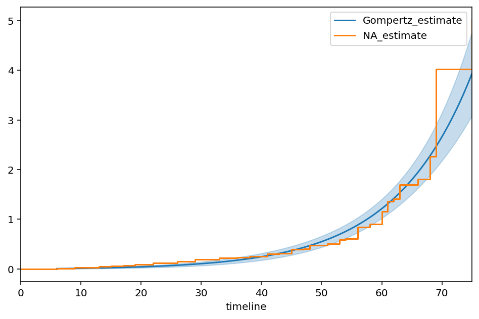
Gompertz
[95]:
class GompertzFitter(ParametricUnivariateFitter):
    # this parameterization is slightly different than wikipedia.
    _fitted_parameter_names = ['nu_', 'b_']

    def _cumulative_hazard(self, params, times):
        nu_, b_ = params
        return nu_ * (np.expm1(times * b_))
[96]:
T, E = waltons['T'], waltons['E']

ggf = GompertzFitter()
ggf.fit(T, E)
ggf.print_summary()
ax = ggf.plot_cumulative_hazard(figsize=(8,5))
ax = NelsonAalenFitter().fit(T, E).plot(ax=ax, ci_show=False)
| model | lifelines.GompertzFitter |
|---|---|
| number of observations | 163 |
| number of events observed | 156 |
| log-likelihood | -650.60 |
| hypothesis | nu_ != 1, b_ != 1 |
| coef | se(coef) | coef lower 95% | coef upper 95% | z | p | -log2(p) | |
|---|---|---|---|---|---|---|---|
| nu_ | 0.01 | 0.00 | 0.00 | 0.02 | -234.94 | <0.005 | inf |
| b_ | 0.08 | 0.01 | 0.07 | 0.09 | -159.07 | <0.005 | inf |
APGW
根据论文《生存分析的灵活参数建模框架》,https://arxiv.org/pdf/1901.03212.pdf
[97]:
class APGWFitter(ParametricUnivariateFitter):
    # this parameterization is slightly different than wikipedia.
    _fitted_parameter_names = ['kappa_', 'gamma_', 'phi_']

    def _cumulative_hazard(self, params, t):
        kappa_, phi_, gamma_ = params
        return (kappa_ + 1) / kappa_ * ((1 + ((phi_ * t) ** gamma_) /(kappa_ + 1)) ** kappa_ -1)
[98]:
apg = APGWFitter()
apg.fit(T, E)
apg.print_summary(2)
ax = apg.plot_cumulative_hazard(figsize=(8,5))
ax = NelsonAalenFitter().fit(T, E).plot(ax=ax, ci_show=False)
| model | lifelines.APGWFitter |
|---|---|
| number of observations | 163 |
| number of events observed | 156 |
| log-likelihood | -655.98 |
| hypothesis | kappa_ != 1, gamma_ != 1, phi_ != 1 |
| coef | se(coef) | coef lower 95% | coef upper 95% | z | p | -log2(p) | |
|---|---|---|---|---|---|---|---|
| kappa_ | 19602.21 | 407112.67 | -778323.96 | 817528.38 | 0.05 | 0.96 | 0.06 |
| gamma_ | 0.02 | 0.00 | 0.02 | 0.02 | -3627.42 | <0.005 | inf |
| phi_ | 2.89 | 0.21 | 2.48 | 3.30 | 9.03 | <0.005 | 62.34 |

使用贝塔分布的有界生命周期
也许你的数据在0和某个(未知)上限M之间?也就是说,寿命不能超过M。也许你知道M,也许你不知道。
[16]:
n = 100
T = 5 * np.random.random(n)**2
T_censor = 10 * np.random.random(n)**2
E = T < T_censor
T_obs = np.minimum(T, T_censor)
[17]:
from autograd_gamma import betainc

class BetaFitter(ParametricUnivariateFitter):
    _fitted_parameter_names = ['alpha_', 'beta_', "m_"]
    _bounds = [(0, None), (0, None), (T.max(), None)]

    def _cumulative_density(self, params, times):
        alpha_, beta_, m_ = params
        return betainc(alpha_, beta_, times / m_)

    def _cumulative_hazard(self, params, times):
        return -np.log(1-self._cumulative_density(params, times))
[18]:
beta_fitter = BetaFitter().fit(T_obs, E)
beta_fitter.plot()
beta_fitter.print_summary()
/Users/camerondavidson-pilon/code/lifelines/lifelines/fitters/__init__.py:936: StatisticalWarning: The diagonal of the variance_matrix_ has negative values. This could be a problem with BetaFitter's fit to the data.

It's advisable to not trust the variances reported, and to be suspicious of the
fitted parameters too. Perform plots of the cumulative hazard to help understand
the latter's bias.

To fix this, try specifying an `initial_point` kwarg in `fit`.

  warnings.warn(warning_text, utils.StatisticalWarning)
/Users/camerondavidson-pilon/code/lifelines/lifelines/fitters/__init__.py:460: RuntimeWarning: invalid value encountered in sqrt
  np.einsum("nj,jk,nk->n", gradient_at_times.T, self.variance_matrix_, gradient_at_times.T)
| model | lifelines.BetaFitter |
|---|---|
| number of observations | 100 |
| number of events observed | 64 |
| log-likelihood | -79.87 |
| hypothesis | alpha_ != 1, beta_ != 1, m_ != 5.92869 |
| coef | se(coef) | coef lower 95% | coef upper 95% | z | p | -log2(p) | |
|---|---|---|---|---|---|---|---|
| alpha_ | 0.53 | 0.06 | 0.40 | 0.65 | -7.34 | <0.005 | 42.10 |
| beta_ | 1.15 | nan | nan | nan | nan | nan | nan |
| m_ | 4.93 | nan | nan | nan | nan | nan | nan |

离散生存模型
到目前为止,我们只研究了连续时间生存模型,其中时间可以取任何正值。如果我们想考虑离散生存时间(例如,在正整数上),我们需要进行一些小的调整。对于离散生存模型,危险和累积危险之间的关系稍微复杂一些。这是因为有两种定义累积危险的方式。
我们也不再具有关系\(h(t) = \frac{d H(t)}{dt}\),因为\(t\)不再是连续的。相反,根据您选择使用的累积风险版本(推断将是相同的),我们必须在lifelines中重新定义风险函数。
Here is an example 这是一个离散生存模型的例子,最初可能看起来不像生存模型,我们在这里使用了一个重新定义的 _hazard 函数。
寻找更多可以构建的示例?请参阅文档中关于时间滞后生存的其他独特生存模型。