估计单变量模型
在之前的部分中,我们介绍了生存分析的应用及其依赖的数学对象。在本文中,我们将使用真实数据和lifelines库来估计这些对象。
使用Kaplan-Meier估计生存函数
在这个例子中,我们将研究世界各地政治领导人的任期。在这种情况下,政治领导人被定义为控制统治政权的个人在任时间。这个政治领导人可以是民选总统、非民选独裁者、君主等。出生事件是个人任期的开始,死亡事件是个人自愿退休。如果他们在a)数据集编制时(2008年)仍在任,或b)在任期间去世(包括被暗杀),则可能会发生审查。
例如,布什政权始于2000年,并于2008年他退休时正式结束,因此该政权的寿命为八年,并且观察到了一个“死亡”事件。另一方面,肯尼迪政权持续了2年,从1961年到1963年,而该政权的正式死亡事件并未被观察到——肯尼迪在正式退休前去世。
(这是一个例子,它愉快地重新定义了出生和死亡事件,实际上通过使用死亡作为审查事件完全颠覆了这个概念。这也是一个例子,其中当前时间不是审查的唯一原因;还有其他替代事件(例如,在任期间死亡)可能是审查的原因。
为了估计生存函数,我们首先将使用Kaplan-Meier估计,定义如下:
其中 \(d_i\) 是在时间 \(t\) 的死亡事件数量,而 \(n_i\) 是在时间 \(t\) 之前有死亡风险的受试者数量。
让我们引入我们的数据集。
from lifelines.datasets import load_dd

data = load_dd()
data.head()
民主 |
制度 |
起始年份 |
持续时间 |
观察到的 |
国家名称 |
cowcode2 |
politycode |
un_region_name |
un_continent_name |
ehead |
leaderspellreg |
|---|---|---|---|---|---|---|---|---|---|---|---|
非民主 |
君主制 |
1946 |
7 |
1 |
阿富汗 |
700 |
700 |
南亚 |
亚洲 |
穆罕默德·查希尔·沙阿 |
穆罕默德·查希尔·沙阿。阿富汗。1946年。1952年。君主制 |
非民主 |
民用词典 |
1953 |
10 |
1 |
阿富汗 |
700 |
700 |
南亚 |
亚洲 |
萨达尔·穆罕默德·达乌德 |
萨达尔·穆罕默德·达乌德。阿富汗。1953年。1962年。文官独裁 |
非民主 |
君主制 |
1963 |
10 |
1 |
阿富汗 |
700 |
700 |
南亚 |
亚洲 |
穆罕默德·查希尔·沙阿 |
穆罕默德·查希尔·沙阿。阿富汗。1963年。1972年。君主制 |
非民主 |
民用词典 |
1973 |
5 |
0 |
阿富汗 |
700 |
700 |
南亚 |
亚洲 |
萨达尔·穆罕默德·达乌德 |
萨达尔·穆罕默德·达乌德。阿富汗。1973年。1977年。平民独裁 |
非民主 |
民用词典 |
1978 |
1 |
0 |
阿富汗 |
700 |
700 |
南亚 |
亚洲 |
努尔·穆罕默德·塔拉基 |
努尔·穆罕默德·塔拉基。阿富汗。1978年。1978年。平民独裁 |
从lifelines库中,我们需要
KaplanMeierFitter来进行这个练习:
from lifelines import KaplanMeierFitter
kmf = KaplanMeierFitter()
注意
下面讨论了在lifelines中估计生存函数的其他方法。
对于这个估计,我们需要每位领导人在职的持续时间,以及他们是否被观察到已经离职(在任期间去世或在2008年仍在任的领导人,这是数据记录的最新日期,没有观察到死亡事件)。
接下来我们使用KaplanMeierFitter方法fit()将模型拟合到数据上。(这与scikit-learn的fit/predict API类似,并受其启发)。
下面我们使用KaplanMeierFitter来拟合我们的数据:
T = data["duration"]
E = data["observed"]

kmf.fit(T, event_observed=E)
调用fit()方法后,KaplanMeierFitter有一个名为survival_function_的属性(再次强调,我们遵循scikit-learn的样式,在所有估计的属性后附加下划线)。该属性是一个Pandas DataFrame,因此我们可以在其上调用plot():
from matplotlib import pyplot as plt


kmf.survival_function_.plot()
plt.title('Survival function of political regimes');
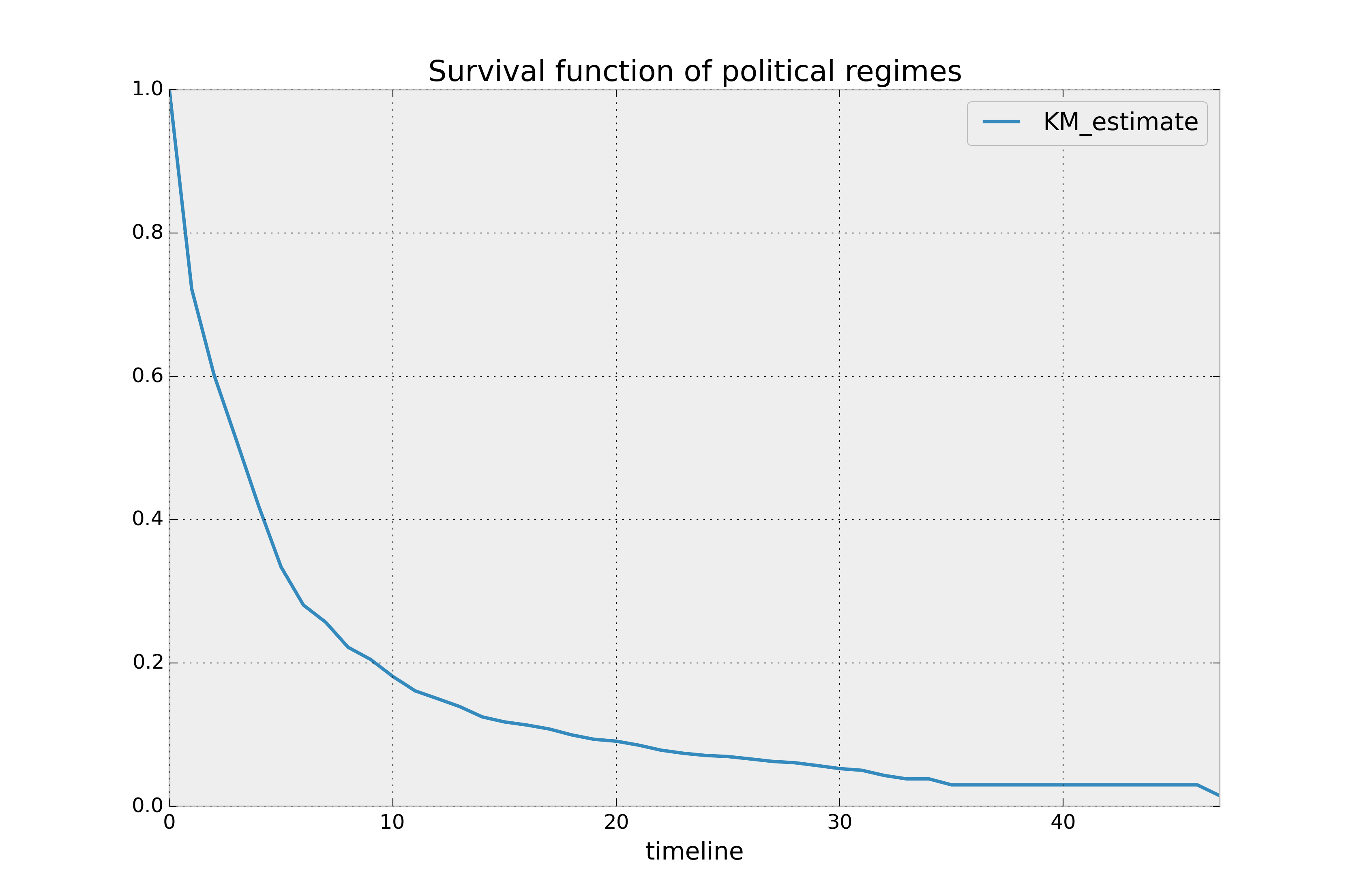
How do we interpret this? The y-axis represents the probability a leader is still
around after \(t\) years, where \(t\) years is on the x-axis. We
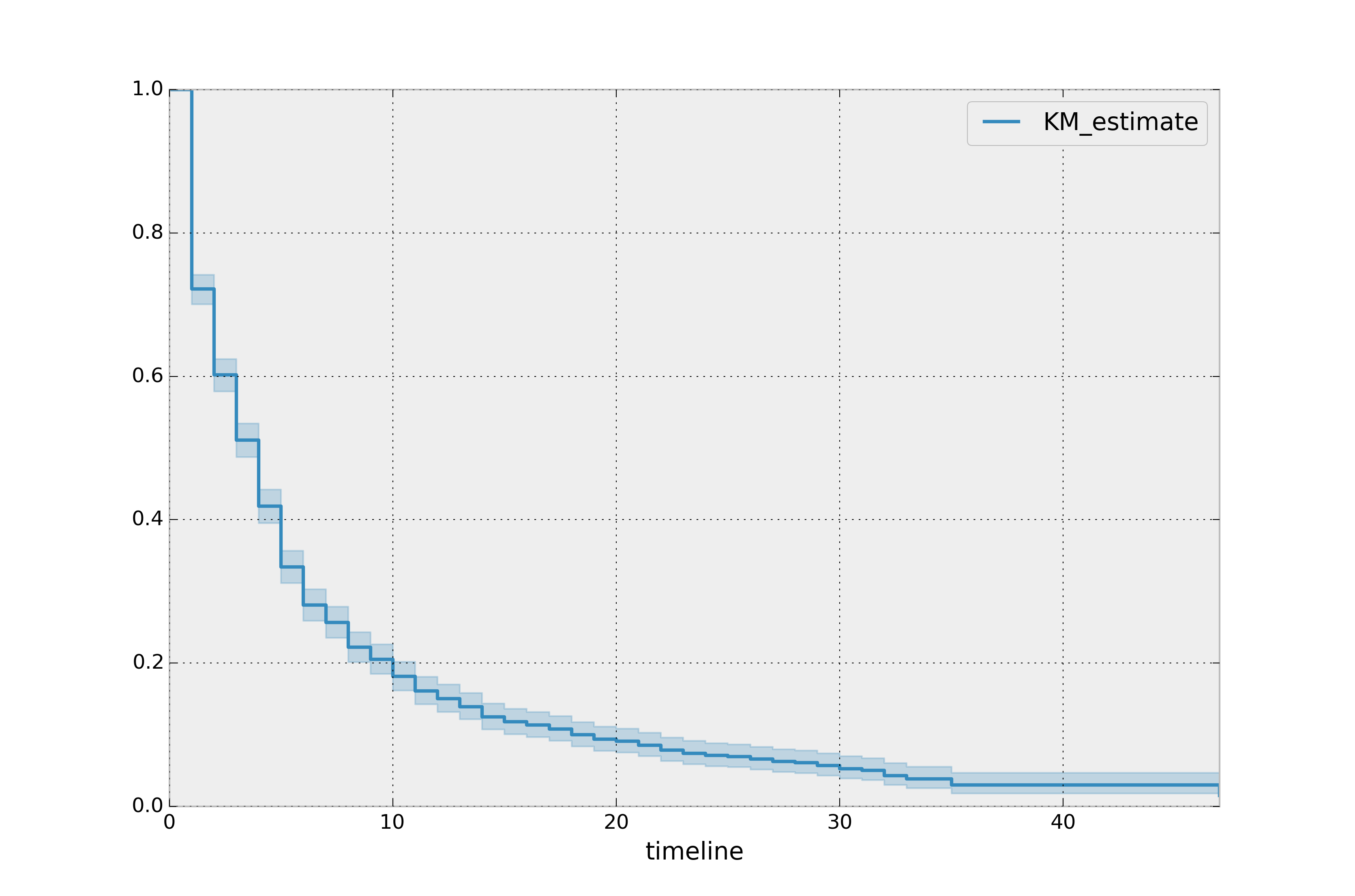
see that very few leaders make it past 20 years in office. Of course, we need to report how uncertain we are about these point estimates, i.e., we need confidence intervals. They are computed in
the call to fit(), and located under the confidence_interval_
property. (The method uses exponential Greenwood confidence interval. The mathematics are found in these notes.) We can call plot() on the KaplanMeierFitter itself to plot both the KM estimate and its confidence intervals:
kmf.plot_survival_function()
中位任期,定义了平均50%的人口已经结束的时间点,是一个属性:
kmf.median_survival_time_
#   4.0
有趣的是,这仅仅是四年。这意味着,在世界各地,当选的领导人 有50%的几率在四年或更短时间内停止任职!要获得中位数的置信区间,你可以使用:
from lifelines.utils import median_survival_times
median_ci = median_survival_times(kmf.confidence_interval_)
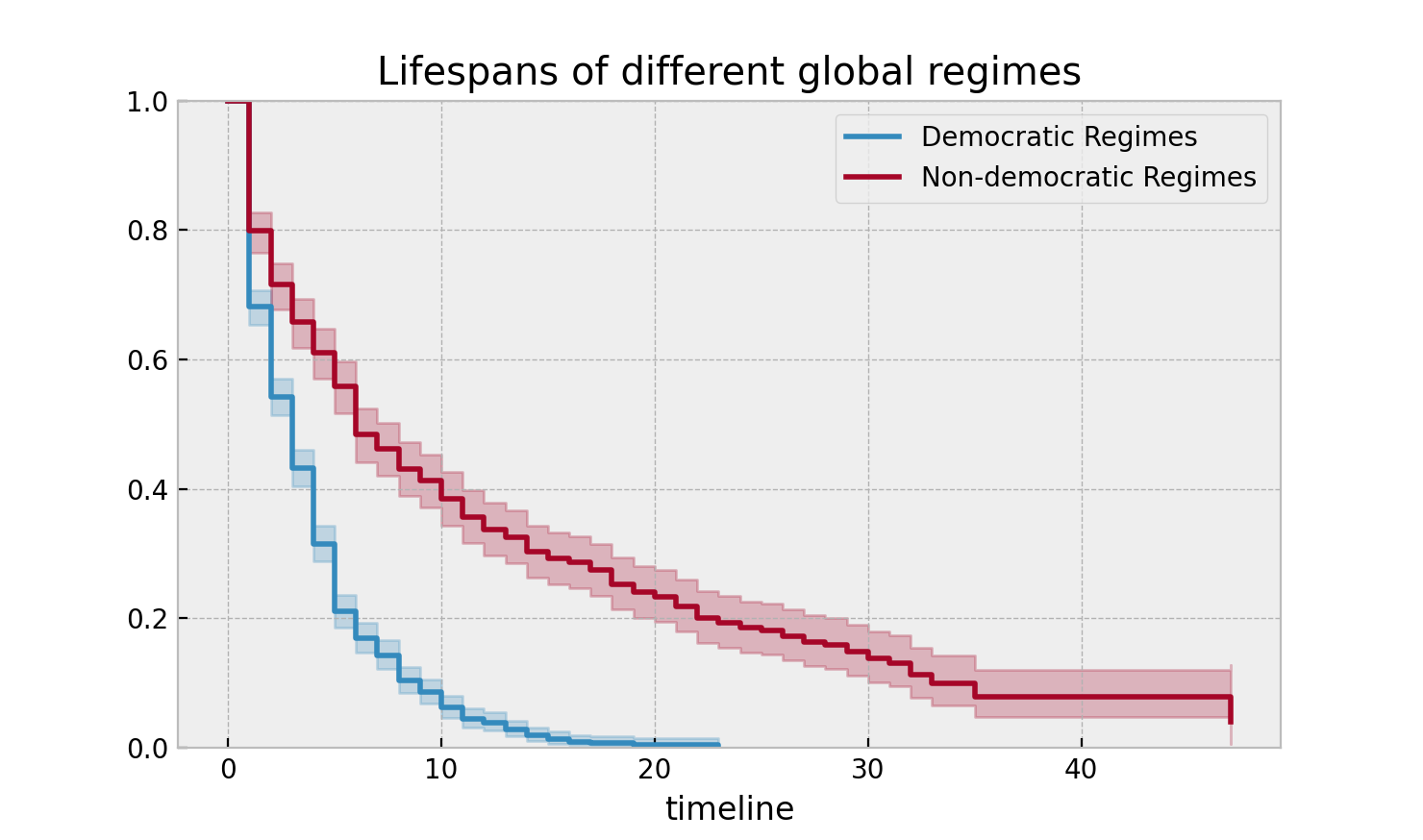
让我们对民主政权与非民主政权进行分段。调用plot在估计本身或拟合器对象上将返回一个axis对象,该对象可用于绘制进一步的估计:
ax = plt.subplot(111)

dem = (data["democracy"] == "Democracy")

kmf.fit(T[dem], event_observed=E[dem], label="Democratic Regimes")
kmf.plot_survival_function(ax=ax)

kmf.fit(T[~dem], event_observed=E[~dem], label="Non-democratic Regimes")
kmf.plot_survival_function(ax=ax)

plt.title("Lifespans of different global regimes");
我们可能对估计某些点之间的概率感兴趣。我们可以使用timeline参数来实现这一点。我们指定感兴趣的时间,并返回一个包含这些时间点生存概率的DataFrame:
import numpy as np

ax = plt.subplot(111)

t = np.linspace(0, 50, 51)
kmf.fit(T[dem], event_observed=E[dem], timeline=t, label="Democratic Regimes")
ax = kmf.plot_survival_function(ax=ax)

kmf.fit(T[~dem], event_observed=E[~dem], timeline=t, label="Non-democratic Regimes")
ax = kmf.plot_survival_function(ax=ax)

plt.title("Lifespans of different global regimes");
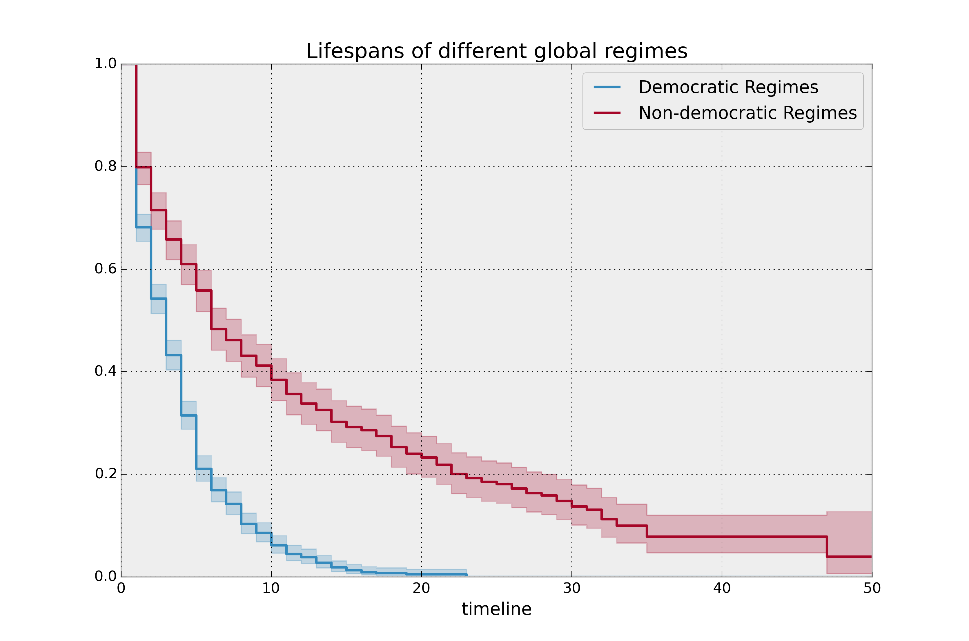
这些非民主政权的存在时间之长令人难以置信。 民主政权确实有一种自然的死亡倾向:无论是通过选举还是自然限制(美国实行严格的八年限制)。 非民主政权的平均寿命大约是民主政权的两倍,但在极端情况下差异明显: 如果你是一个非民主领导人,并且你已经度过了10年的标志,你可能还有很长的寿命。与此同时,民主领导人很少能超过十年,而且在那之后的寿命非常短。
这里生存函数之间的差异非常明显,进行统计测试似乎有些迂腐。如果曲线更相似,或者我们拥有的数据较少,我们可能对进行统计测试感兴趣。在这种情况下,lifelines 包含了在 lifelines.statistics 中的例程来比较两个生存函数。下面我们演示这个例程。函数 lifelines.statistics.logrank_test() 是生存分析中常见的统计测试,用于比较两个事件序列的生成器。如果返回的值超过某个预先指定的值,那么我们判定这两个序列具有不同的生成器。
from lifelines.statistics import logrank_test

results = logrank_test(T[dem], T[~dem], E[dem], E[~dem], alpha=.99)

results.print_summary()

"""
<lifelines.StatisticalResult>
             t_0 = -1
null_distribution = chi squared
degrees_of_freedom = 1
           alpha = 0.99

---
test_statistic      p  -log2(p)
       260.47  <0.005    192.23
"""
有替代的(有时更好的)生存函数测试,我们在这里解释更多:Statistically compare two populations
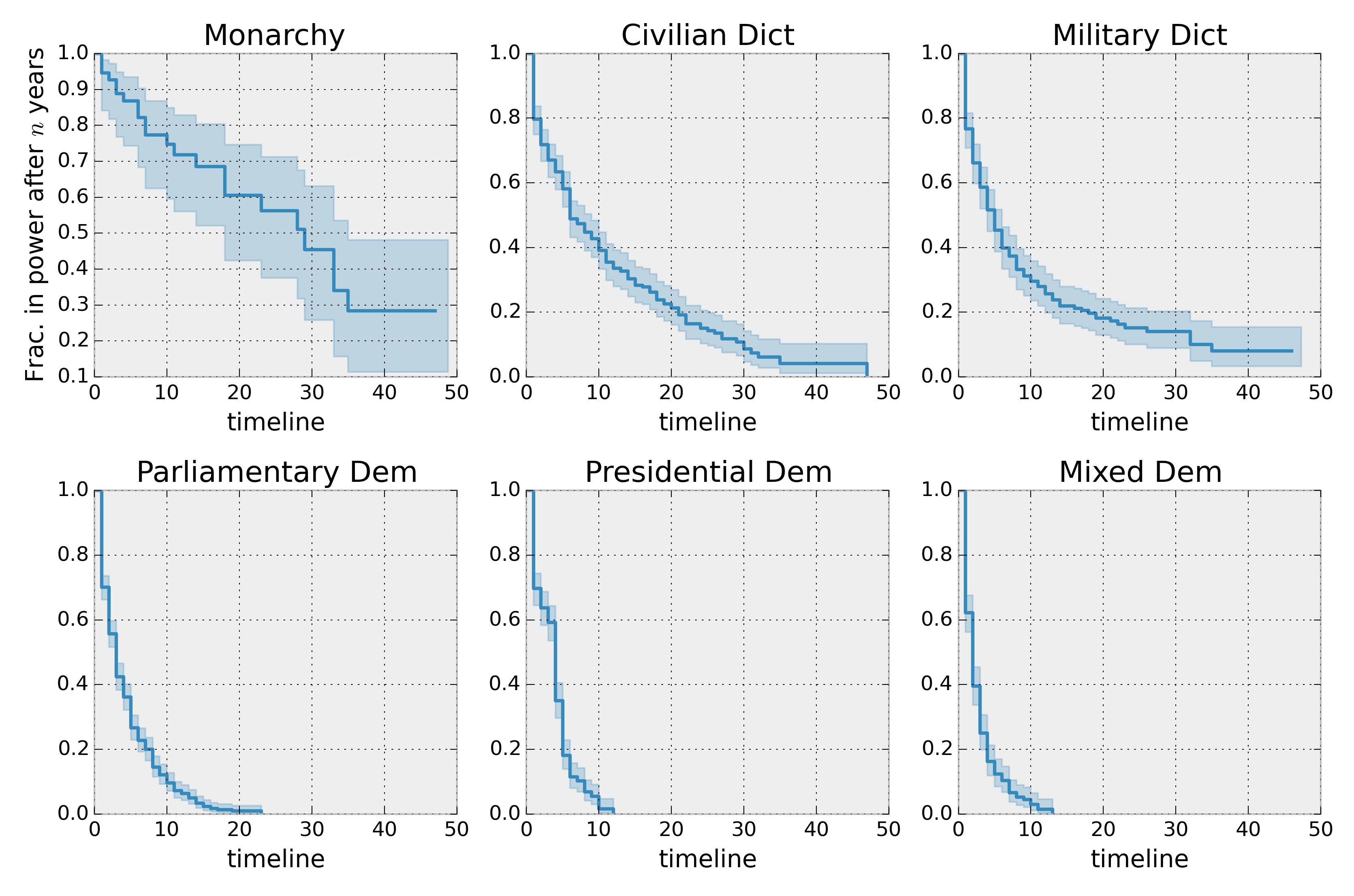
让我们比较数据集中存在的不同类型的制度:
regime_types = data['regime'].unique()

for i, regime_type in enumerate(regime_types):
    ax = plt.subplot(2, 3, i + 1)

    ix = data['regime'] == regime_type
    kmf.fit(T[ix], E[ix], label=regime_type)
    kmf.plot_survival_function(ax=ax, legend=False)

    plt.title(regime_type)
    plt.xlim(0, 50)

    if i==0:
        plt.ylabel('Frac. in power after $n$ years')

plt.tight_layout()
展示Kaplan Meier图的最佳实践
最近对统计学家、医疗专业人员和其他利益相关者的一项调查表明,添加两个信息,即汇总表和置信区间,大大提高了Kaplan Meier图的有效性,参见“Morris TP, Jarvis CI, Cragg W, et al. Proposals on Kaplan–Meier plots in medical research and a survey of stakeholder views: KMunicate. BMJ Open 2019;9:e030215. doi:10.1136/bmjopen-2019-030215”。
在lifelines中,置信区间会自动添加,但也有at_risk_counts参数可以添加摘要表:
kmf = KaplanMeierFitter().fit(T, E, label="all_regimes")
kmf.plot_survival_function(at_risk_counts=True)
plt.tight_layout()
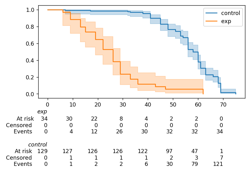
有关更多详细信息以及如何将其扩展到多条曲线,请参阅此处文档。
将数据转换为正确的格式
lifelines 的数据格式在所有估计器类和函数中是一致的:一个个体持续时间的数组,以及个体的事件观察(如果有的话)。这些通常分别表示为 T 和 E。例如:
T = [0, 3, 3, 2, 1, 2]
E = [1, 1, 0, 0, 1, 1]
kmf.fit(T, event_observed=E)
原始数据并不总是以这种格式提供——lifelines 包含一些辅助函数,可以将数据格式转换为 lifelines 格式。这些函数位于 lifelines.utils 子库中。例如,函数 datetimes_to_durations() 接受一个开始时间/日期的数组或 Pandas 对象,以及一个结束时间/日期的数组或 Pandas 对象(如果未观察到则为 None):
from lifelines.utils import datetimes_to_durations

start_date = ['2013-10-10 0:00:00', '2013-10-09', '2013-10-10']
end_date = ['2013-10-13', '2013-10-10', None]
T, E = datetimes_to_durations(start_date, end_date, fill_date='2013-10-15')
print('T (durations): ', T)
print('E (event_observed): ', E)
T (durations):  [ 3.  1.  5.]
E (event_observed):  [ True  True False]
函数 datetimes_to_durations() 非常灵活,并且有许多关键字可以调整。
使用Nelson-Aalen估计风险率
生存函数是总结和可视化生存数据集的一个很好的方法,然而它并不是唯一的方法。如果我们对人群的风险函数\(h(t)\)感到好奇,不幸的是,我们无法转换Kaplan Meier估计——统计学并不完全那样工作。幸运的是,有一个适当的非参数估计器用于累积风险函数\(H(t)\):
这个量的估计器被称为Nelson Aalen估计器:
其中 \(d_i\) 是在时间 \(t_i\) 的死亡人数, \(n_i\) 是易感个体的数量。
在lifelines中,此估计器可作为NelsonAalenFitter使用。让我们使用上面的政权数据集:
T = data["duration"]
E = data["observed"]

from lifelines import NelsonAalenFitter
naf = NelsonAalenFitter()

naf.fit(T,event_observed=E)
拟合后,类暴露了属性 cumulative_hazard_`() 作为
一个 DataFrame:
print(naf.cumulative_hazard_.head())
naf.plot_cumulative_hazard()
   NA-estimate
0     0.000000
1     0.325912
2     0.507356
3     0.671251
4     0.869867

[5 rows x 1 columns]
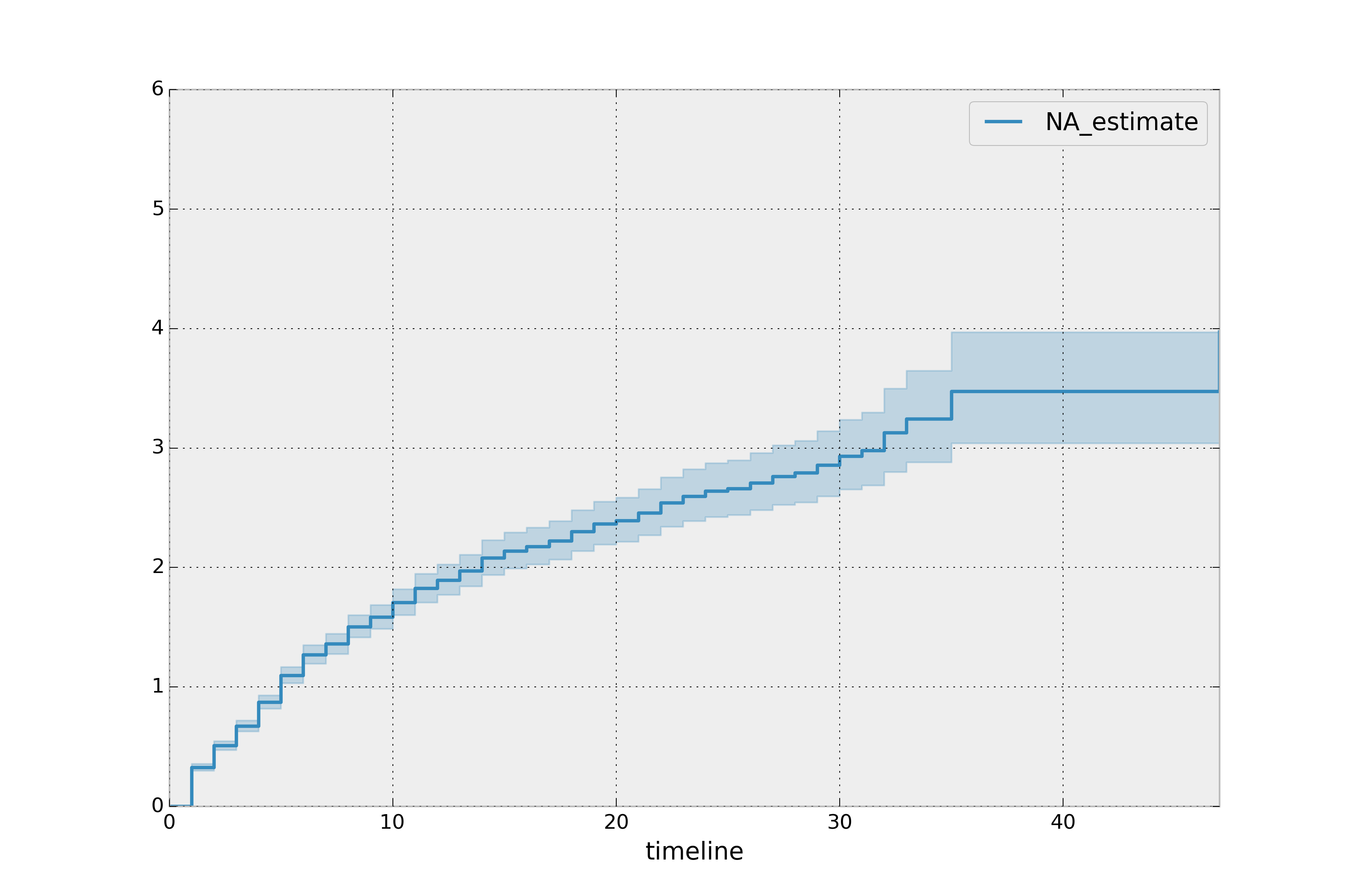
累积风险函数比生存函数更难理解,但风险函数是生存分析中更高级技术的基础。回想一下,我们正在估计累积风险函数,\(H(t)\)。(为什么?估计的总和比逐点估计要稳定得多。)因此,我们知道这条曲线的变化率是风险函数的估计。
观察上图,危险似乎一开始很高,然后逐渐减小(从变化率的下降可以看出)。让我们在前20年期间,将民主和非民主政权分开来看:
注意
我们在这里使用loc参数调用plot_cumulative_hazard:它接受一个slice并仅绘制该切片内的点。
naf.fit(T[dem], event_observed=E[dem], label="Democratic Regimes")
ax = naf.plot_cumulative_hazard(loc=slice(0, 20))

naf.fit(T[~dem], event_observed=E[~dem], label="Non-democratic Regimes")
naf.plot_cumulative_hazard(ax=ax, loc=slice(0, 20))

plt.title("Cumulative hazard function of different global regimes");
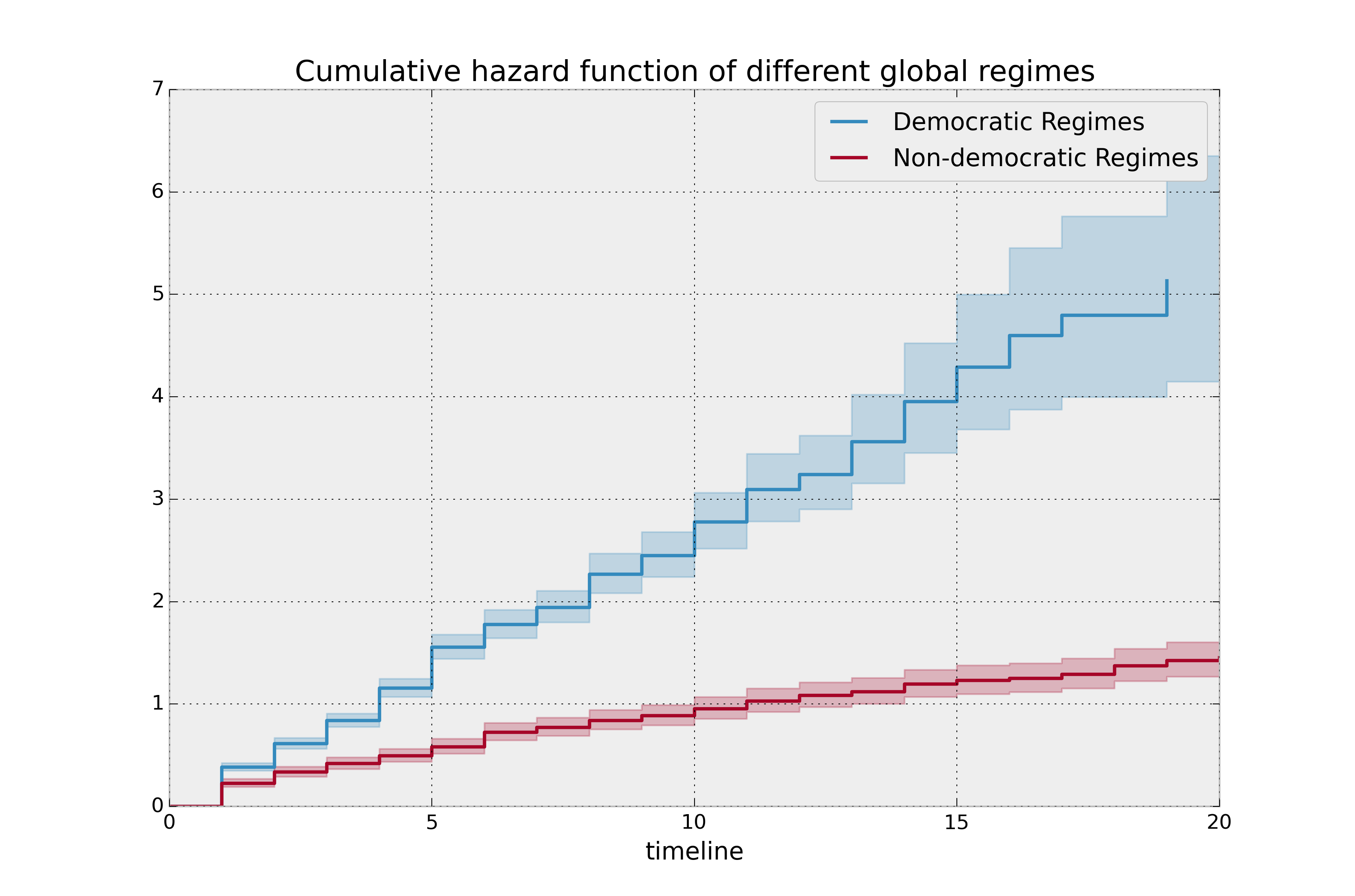
观察变化率,我会说两种政治哲学都有恒定的风险,尽管民主政体的恒定风险要高得多。
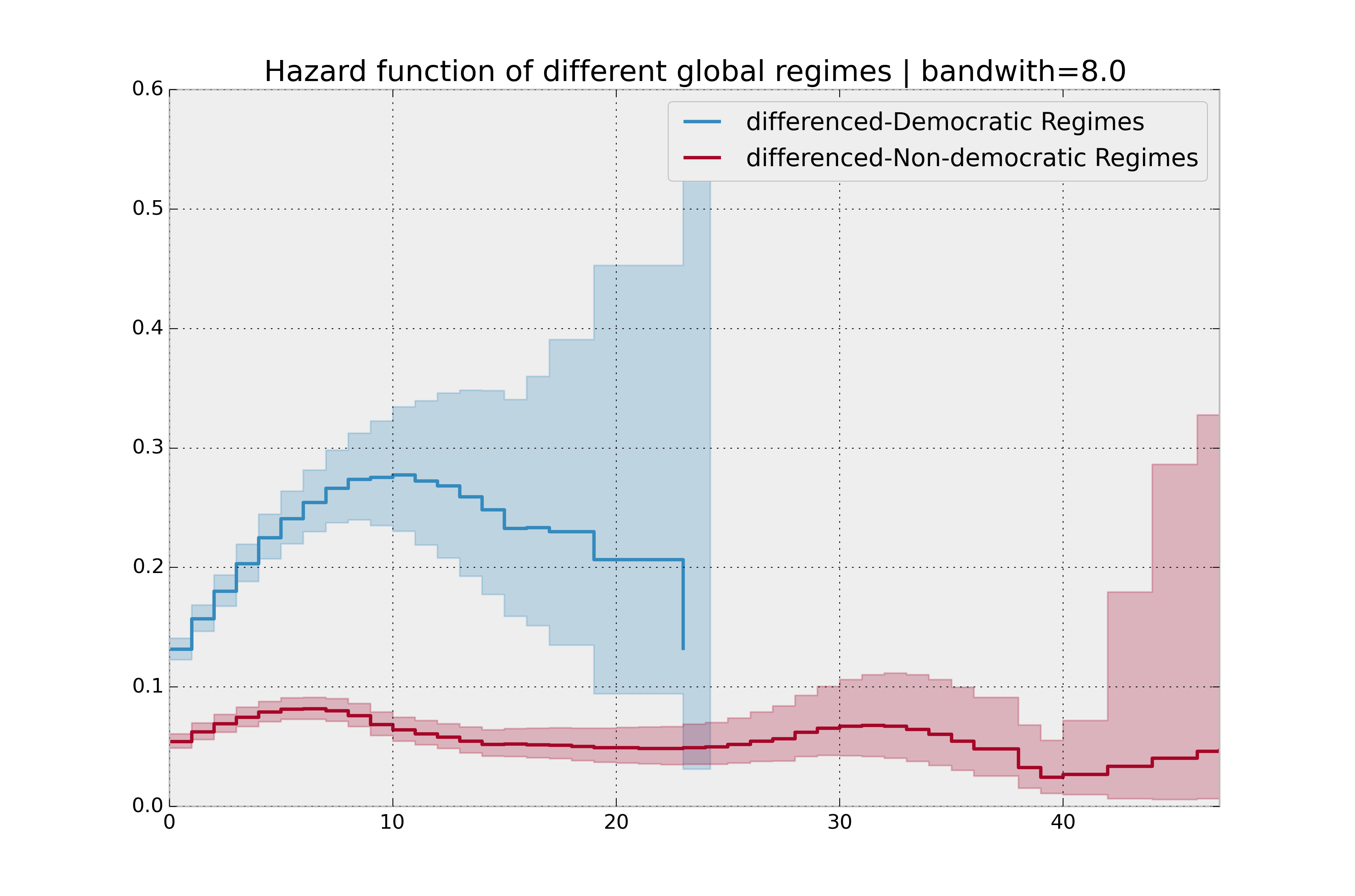
平滑风险函数
累积风险函数的解释可能比较困难——这不是我们通常解释函数的方式。另一方面,大多数生存分析都是使用累积风险函数进行的,因此建议理解它。
或者,我们可以推导出更易解释的风险函数,但有一个问题。推导过程涉及到一个核平滑器(用于平滑累积风险函数的差异),这需要我们指定一个控制平滑量的带宽参数。这个功能在smoothed_hazard_()和smoothed_hazard_confidence_intervals_()方法中。为什么是方法?它们需要一个表示带宽的参数。
还有一个plot_hazard()函数(也需要一个bandwidth关键字),它将绘制估计值加上置信区间,类似于传统的plot()功能。
bandwidth = 3.

naf.fit(T[dem], event_observed=E[dem], label="Democratic Regimes")
ax = naf.plot_hazard(bandwidth=bandwidth)

naf.fit(T[~dem], event_observed=E[~dem], label="Non-democratic Regimes")
naf.plot_hazard(ax=ax, bandwidth=bandwidth)

plt.title("Hazard function of different global regimes | bandwidth=%.1f" % bandwidth);
plt.ylim(0, 0.4)
plt.xlim(0, 25);

这里更清楚地看出哪个群体的风险更高,非民主政体似乎具有恒定的风险。
没有明显的方法来选择带宽,不同的带宽会产生不同的推断,因此在这里要非常小心。我的建议:坚持使用累积风险函数。
bandwidth = 8.0

naf.fit(T[dem], event_observed=E[dem], label="Democratic Regimes")
ax = naf.plot_hazard(bandwidth=bandwidth)

naf.fit(T[~dem], event_observed=E[~dem], label="Non-democratic Regimes")
naf.plot_hazard(ax=ax, bandwidth=bandwidth)

plt.title("Hazard function of different global regimes | bandwidth=%.1f" % bandwidth);
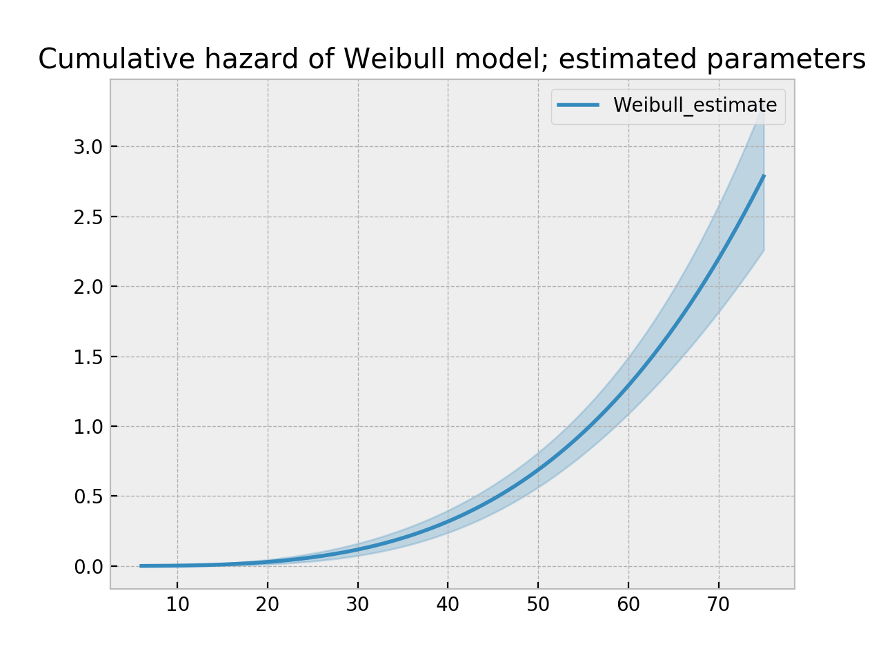
使用参数模型估计累积风险
拟合到威布尔模型
另一个非常流行的生存数据模型是Weibull模型。与Nelson-Aalen估计器相比,这个模型是一个参数模型,意味着它有一个函数形式,并且有我们正在拟合数据的参数。(Nelson-Aalen估计器没有需要拟合的参数)。生存函数如下所示:
先验地,我们不知道\(\lambda\)和\(\rho\)是什么,但我们使用手头的数据来估计这些参数。我们建模并估计累积风险率而不是生存函数(这与Kaplan-Meier估计器不同):
在lifelines中,可以使用WeibullFitter类进行估计。plot()方法将绘制累积风险。
from lifelines import WeibullFitter
from lifelines.datasets import load_waltons

data = load_waltons()

T = data['T']
E = data['E']

wf = WeibullFitter().fit(T, E)

wf.print_summary()
ax = wf.plot_cumulative_hazard()
ax.set_title("Cumulative hazard of Weibull model; estimated parameters")


"""
<lifelines.WeibullFitter: fitted with 163 observations, 7 censored>
number of subjects = 163
  number of events = 156
    log-likelihood = -672.062
        hypothesis = lambda != 1, rho != 1

---
         coef  se(coef)  lower 0.95  upper 0.95      p  -log2(p)
lambda_  0.02      0.00        0.02        0.02 <0.005       inf
rho_     3.45      0.24        2.97        3.93 <0.005     76.83
"""
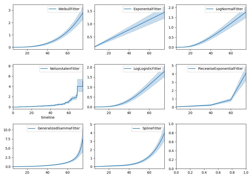
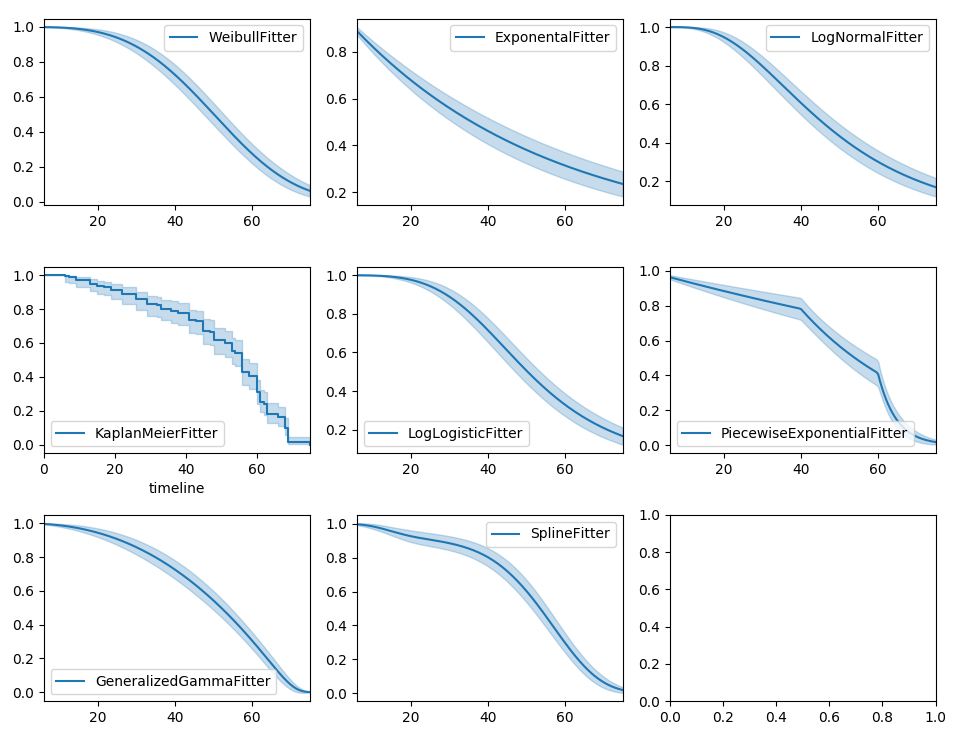
其他参数模型:指数、对数逻辑、对数正态和样条
同样地,在lifelines中还有其他参数模型。通常,选择哪种参数模型是由对持续时间分布的知识或某种模型拟合优度决定的。以下是相同数据的内置参数模型和Nelson-Aalen非参数模型。
from lifelines import (WeibullFitter, ExponentialFitter,
LogNormalFitter, LogLogisticFitter, NelsonAalenFitter,
PiecewiseExponentialFitter, GeneralizedGammaFitter, SplineFitter)

from lifelines.datasets import load_waltons
data = load_waltons()

fig, axes = plt.subplots(3, 3, figsize=(10, 7.5))

T = data['T']
E = data['E']

wbf = WeibullFitter().fit(T, E, label='WeibullFitter')
exf = ExponentialFitter().fit(T, E, label='ExponentialFitter')
lnf = LogNormalFitter().fit(T, E, label='LogNormalFitter')
naf = NelsonAalenFitter().fit(T, E, label='NelsonAalenFitter')
llf = LogLogisticFitter().fit(T, E, label='LogLogisticFitter')
pwf = PiecewiseExponentialFitter([40, 60]).fit(T, E, label='PiecewiseExponentialFitter')
gg = GeneralizedGammaFitter().fit(T, E, label='GeneralizedGammaFitter')
spf = SplineFitter([6, 20, 40, 75]).fit(T, E, label='SplineFitter')

wbf.plot_cumulative_hazard(ax=axes[0][0])
exf.plot_cumulative_hazard(ax=axes[0][1])
lnf.plot_cumulative_hazard(ax=axes[0][2])
naf.plot_cumulative_hazard(ax=axes[1][0])
llf.plot_cumulative_hazard(ax=axes[1][1])
pwf.plot_cumulative_hazard(ax=axes[1][2])
gg.plot_cumulative_hazard(ax=axes[2][0])
spf.plot_cumulative_hazard(ax=axes[2][1])
lifelines 也可以用来定义你自己的参数模型。有一个关于此的教程可用,参见 分段指数模型和创建自定义模型。
参数模型也可以用来创建和绘制生存函数。下面我们将参数模型与非参数的Kaplan-Meier估计进行比较:
from lifelines import KaplanMeierFitter

fig, axes = plt.subplots(3, 3, figsize=(10, 7.5))

T = data['T']
E = data['E']

kmf = KaplanMeierFitter().fit(T, E, label='KaplanMeierFitter')
wbf = WeibullFitter().fit(T, E, label='WeibullFitter')
exf = ExponentialFitter().fit(T, E, label='ExponentialFitter')
lnf = LogNormalFitter().fit(T, E, label='LogNormalFitter')
llf = LogLogisticFitter().fit(T, E, label='LogLogisticFitter')
pwf = PiecewiseExponentialFitter([40, 60]).fit(T, E, label='PiecewiseExponentialFitter')
gg = GeneralizedGammaFitter().fit(T, E, label='GeneralizedGammaFitter')
spf = SplineFitter([6, 20, 40, 75]).fit(T, E, label='SplineFitter')

wbf.plot_survival_function(ax=axes[0][0])
exf.plot_survival_function(ax=axes[0][1])
lnf.plot_survival_function(ax=axes[0][2])
kmf.plot_survival_function(ax=axes[1][0])
llf.plot_survival_function(ax=axes[1][1])
pwf.plot_survival_function(ax=axes[1][2])
gg.plot_survival_function(ax=axes[2][0])
spf.plot_survival_function(ax=axes[2][1])
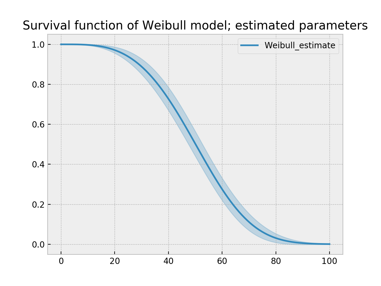
使用参数模型,我们有一个函数形式,允许我们将生存函数(或风险或累积风险)扩展到我们观察到的最大持续时间之后。这被称为外推。我们可以通过几种方式做到这一点。
timeline = np.linspace(0, 100, 200)

# directly compute the survival function, these return a pandas Series
wbf = WeibullFitter().fit(T, E)
wbf.survival_function_at_times(timeline)
wbf.hazard_at_times(timeline)
wbf.cumulative_hazard_at_times(timeline)

# use the `timeline` kwarg in `fit`
# by default, all functions and properties will use
# these values provided
wbf = WeibullFitter().fit(T, E, timeline=timeline)

ax = wbf.plot_survival_function()
ax.set_title("Survival function of Weibull model; estimated parameters")
模型选择
当基础数据生成分布未知时,我们依赖于拟合度量来判断哪个模型最合适。lifelines 提供了QQ图,使用QQ图选择参数模型,以及比较AIC和其他度量的工具:使用AIC选择参数模型。
其他类型的审查
左删失数据和非检测
我们主要关注的是右删失,它描述了我们没有观察到死亡事件的情况。这种情况是最常见的。另外,还有一些情况是我们没有观察到出生事件的发生。考虑一个医生看到某种潜在疾病的症状延迟出现的情况。医生不确定疾病是何时被感染的(出生),但知道它是在发现之前发生的。
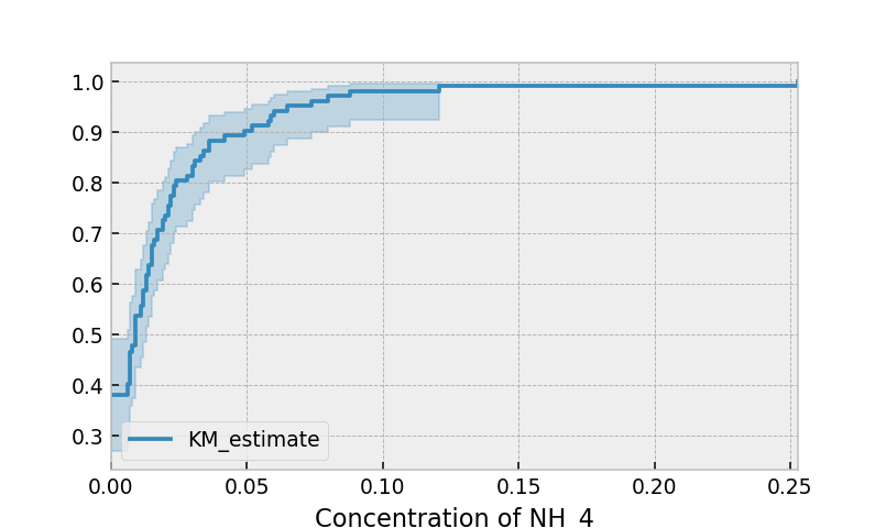
另一种我们遇到左删失数据的情况是,测量结果只有上限,也就是说,测量仪器只能检测到测量结果小于某个上限。这个上限通常被称为检测限(LOD)。实际上,可能存在多个LOD。一个非常重要的统计学教训是:不要天真地“填补”这个值。虽然使用LOD的一半之类的值很诱人,但这会在后续分析中引起大量的偏差。以下是一个示例数据集:
注意
在0.21.0版本中,使用参数模型建模左删失数据的推荐API发生了变化。以下是推荐的API。
from lifelines.datasets import load_nh4
df = load_nh4()[['NH4.Orig.mg.per.L', 'NH4.mg.per.L', 'Censored']]
print(df.head())

"""
  NH4.Orig.mg.per.L  NH4.mg.per.L  Censored
1            <0.006         0.006      True
2            <0.006         0.006      True
3             0.006         0.006     False
4             0.016         0.016     False
5            <0.006         0.006      True
"""
lifelines 在大多数单变量模型中支持左删失数据集,包括 KaplanMeierFitter 类,通过使用 fit_left_censoring() 方法。
T, E = df['NH4.mg.per.L'], ~df['Censored']

kmf = KaplanMeierFitter()
kmf.fit_left_censoring(T, E)
与生成生存函数不同,左截尾数据分析更关注累积密度函数。在拟合数据后,这可以通过cumulative_density_属性获得。
print(kmf.cumulative_density_.head())

kmf.plot_cumulative_density() #will plot the CDF
plt.xlabel("Concentration of NH_4")

"""
          KM_estimate
timeline
0.000        0.379897
0.006        0.401002
0.007        0.464319
0.008        0.478828
0.009        0.536868
"""
或者,您可以使用参数模型来建模数据。这允许您“窥视”低于LOD的数据,但使用参数模型意味着您需要正确指定分布。您可以使用像qq图这样的图表来帮助排除某些分布,请参阅使用QQ图选择参数模型和使用AIC选择参数模型。
from lifelines import *
from lifelines.plotting import qq_plot

fig, axes = plt.subplots(3, 2, figsize=(9, 9))
timeline = np.linspace(0, 0.25, 100)

wf = WeibullFitter().fit_left_censoring(T, E, label="Weibull", timeline=timeline)
lnf = LogNormalFitter().fit_left_censoring(T, E, label="Log Normal", timeline=timeline)
lgf = LogLogisticFitter().fit_left_censoring(T, E, label="Log Logistic", timeline=timeline)

# plot what we just fit, along with the KMF estimate
kmf.plot_cumulative_density(ax=axes[0][0], ci_show=False)
wf.plot_cumulative_density(ax=axes[0][0], ci_show=False)
qq_plot(wf, ax=axes[0][1])

kmf.plot_cumulative_density(ax=axes[1][0], ci_show=False)
lnf.plot_cumulative_density(ax=axes[1][0], ci_show=False)
qq_plot(lnf, ax=axes[1][1])

kmf.plot_cumulative_density(ax=axes[2][0], ci_show=False)
lgf.plot_cumulative_density(ax=axes[2][0], ci_show=False)
qq_plot(lgf, ax=axes[2][1])
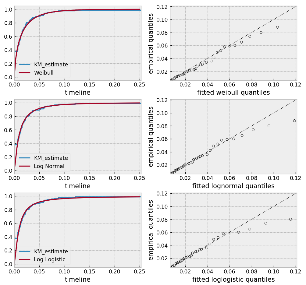
基于以上分析,对数正态分布似乎拟合得很好,而威布尔分布则完全不适合。
区间删失数据
数据也可以是区间截尾的。一个例子是定期记录一群生物的数量。它们的死亡是区间截尾的,因为你知道一个个体在两个观察期之间死亡。
from lifelines.datasets import load_diabetes
from lifelines.plotting import plot_interval_censored_lifetimes

df = load_diabetes()
plot_interval_censored_lifetimes(df['left'], df['right'])
在上面,我们可以看到一些受试者的死亡时间被准确观察到(用红色●表示),而一些受试者的死亡时间在两个时间之间(用红色▶︎和◀︎之间的间隔表示)。我们可以使用任何模型对数据进行推断。注意使用fit_interval_censoring而不是fit。
注意
fit_interval_censoring 的 API 与右删失和左删失数据不同。
wf = WeibullFitter()
wf.fit_interval_censoring(lower_bound=df['left'], upper_bound=df['right'])

# or, a non-parametric estimator:
# for now, this assumes closed observation intervals, ex: [4,5], not (4, 5) or (4, 5]
kmf = KaplanMeierFitter()
kmf.fit_interval_censoring(df['left'], df['right'])

ax = kmf.plot_survival_function()
wf.plot_survival_function(ax=ax)
另一个使用lifelines处理区间删失数据的例子位于这里。
左截断(延迟进入)数据
另一种引入数据集的偏差形式称为左截断(或晚期进入)。左截断可能发生在许多情况下。一种情况是,个体可能在进入研究之前有机会死亡。例如,如果你正在测量监狱中囚犯的死亡时间,囚犯将在不同年龄进入研究。因此,可能存在一些反事实的个体,他们本应进入你的研究(即入狱),但却提前死亡。
所有的拟合器,如KaplanMeierFitter和任何参数模型,都有一个可选的参数entry,它是一个与持续时间数组大小相等的数组。它描述了从实际的“出生”(或“暴露”)到进入研究的时间。
注意
持续时间数组中没有变化:它仍然测量从“出生”到退出研究(无论是死亡还是审查)的时间。也就是说,持续时间指的是绝对死亡时间,而不是相对于研究入组的持续时间。
另一种左截断的情况发生在研究对象在进入研究之前就已经暴露。例如,一项关于艾滋病患者全因死亡率的研究,招募了之前被诊断为艾滋病的个体,可能是在几年前。在下面的例子中,我们将使用一个类似的数据集,称为多中心艾滋病队列研究。在下图中,我们绘制了研究对象的生存时间。实线表示研究对象在我们的观察期内,虚线表示诊断和研究进入之间的未观察期。线末端的实心点代表死亡。
from lifelines.datasets import load_multicenter_aids_cohort_study
from lifelines.plotting import plot_lifetimes

df = load_multicenter_aids_cohort_study()

plot_lifetimes(
    df["T"],
    event_observed=df["D"],
    entry=df["W"],
    event_observed_color="#383838",
    event_censored_color="#383838",
    left_truncated=True,
)
plt.ylabel("Patient Number")
plt.xlabel("Years from AIDS diagnosis")
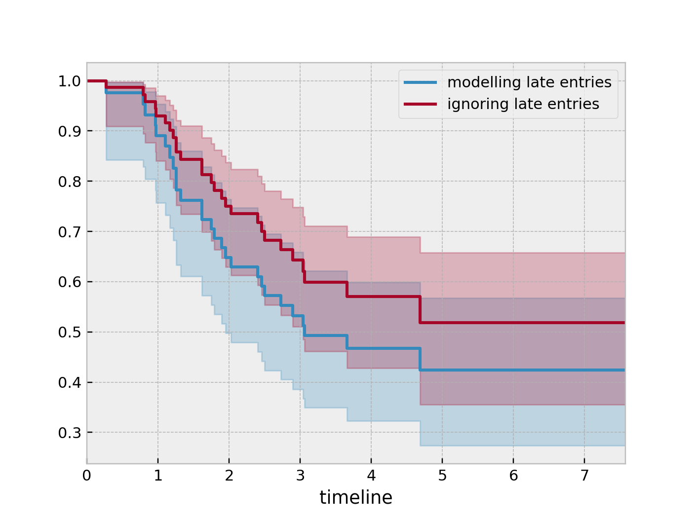
因此,受试者#77,即顶部的受试者,在7.5年前被诊断出患有艾滋病,但在前4.5年没有参与我们的研究。从这个角度来看,为什么我们不能“填补”虚线并说,例如,“受试者#77活了7.5年”?如果我们这样做,我们将严重低估诊断后早期死亡的机会。为什么?有可能有些人在被诊断后不久就去世了,从未有机会进入我们的研究。然而,如果我们确实设法观察到了他们,他们会在早期压低生存函数。因此,“填补”虚线会使我们对诊断后早期发生的情况过于自信。我们可以在下面看到这一点,当我们建模生存函数时,考虑和不考虑晚期进入的情况。
from lifelines import KaplanMeierFitter

kmf = KaplanMeierFitter()
kmf.fit(df["T"], event_observed=df["D"], entry=df["W"], label='modeling late entries')
ax = kmf.plot_survival_function()

kmf.fit(df["T"], event_observed=df["D"], label='ignoring late entries')
kmf.plot_survival_function(ax=ax)