---

生存回归

通常，除了持续时间之外，我们还有其他想要使用的数据。 这种技术被称为生存回归——这个名字意味着 我们将协变量（例如，年龄、国家等）回归到 另一个变量——在这种情况下是持续时间。类似于 本教程第一部分中的逻辑，由于存在截尾， 我们不能使用像线性回归这样的传统方法。

生存回归中有几种流行的模型：Cox模型、加速失效模型和Aalen的加性模型。所有模型都试图将风险率\(h(t | x)\)表示为\(t\)和一些协变量\(x\)的函数。我们接下来将探讨这些模型。

回归数据集

生存回归所需的数据集必须为Pandas DataFrame格式。DataFrame的每一行代表一个观察值。应该有一列表示观察值的持续时间。可能（或可能没有）有一列表示每个观察值的事件状态（如果事件发生则为1，如果被审查则为0）。还有您希望回归的其他协变量。可选地，DataFrame中可能有用于分层、权重和聚类的列，这些将在本教程的后面讨论。

我们将使用的一个示例数据集是Rossi再犯数据集，在lifelines中可用作load_rossi()。

from lifelines.datasets import load_rossi

rossi = load_rossi()

"""
     week  arrest  fin  age  race  wexp  mar  paro  prio
0      20       1    0   27     1     0    0     1     3
1      17       1    0   18     1     0    0     1     8
2      25       1    0   19     0     1    0     1    13
3      52       0    1   23     1     1    1     1     1
"""

DataFrame rossi 包含432个观测值。week 列是持续时间，arrest 列表示事件（重新逮捕）是否发生，其他列代表我们希望进行回归的变量。

Cox比例风险模型

Cox比例风险模型背后的思想是，个体的对数风险是其协变量的线性函数以及随时间变化的人群水平基线风险。数学上表示为：

\[\underbrace{h(t | x)}_{\text{hazard}} = \overbrace{b_0(t)}^{\text{baseline hazard}} \underbrace{\exp \overbrace{\left(\sum_{i=1}^n b_i (x_i - \overline{x_i})\right)}^{\text{log-partial hazard}}}_ {\text{partial hazard}}\]

注意这个模型的几个行为：唯一的时间组件在基线风险中，\(b_0(t)\)。在上述方程中，部分风险是一个时间不变的标量因子，只会增加或减少基线风险。因此，协变量的变化只会放大或缩小基线风险。

注意

在其他回归模型中，可能会添加一列1来表示截距或基线。在Cox模型中，这是不必要的。事实上，Cox模型中没有截距——基线风险代表了这一点。如果您的数据集或公式中存在一列1，lifelines 会发出警告，并可能遇到收敛错误。

拟合回归

在lifelines中，Cox模型的实现位于CoxPHFitter下。我们使用fit()将模型拟合到数据集。它有一个print_summary()函数，可以打印系数和相关统计数据的表格视图。

from lifelines import CoxPHFitter
from lifelines.datasets import load_rossi

rossi = load_rossi()

cph = CoxPHFitter()
cph.fit(rossi, duration_col='week', event_col='arrest')

cph.print_summary()  # access the individual results using cph.summary

"""
<lifelines.CoxPHFitter: fitted with 432 total observations, 318 right-censored observations>
             duration col = 'week'
                event col = 'arrest'
   number of observations = 432
number of events observed = 114
   partial log-likelihood = -658.75
         time fit was run = 2019-10-05 14:24:44 UTC

---
       coef  exp(coef)   se(coef)   coef lower 95%   coef upper 95%  exp(coef) lower 95%  exp(coef) upper 95%
fin   -0.38       0.68       0.19            -0.75            -0.00                 0.47                 1.00
age   -0.06       0.94       0.02            -0.10            -0.01                 0.90                 0.99
race   0.31       1.37       0.31            -0.29             0.92                 0.75                 2.50
wexp  -0.15       0.86       0.21            -0.57             0.27                 0.57                 1.30
mar   -0.43       0.65       0.38            -1.18             0.31                 0.31                 1.37
paro  -0.08       0.92       0.20            -0.47             0.30                 0.63                 1.35
prio   0.09       1.10       0.03             0.04             0.15                 1.04                 1.16

         z      p   -log2(p)
fin  -1.98   0.05       4.40
age  -2.61   0.01       6.79
race  1.02   0.31       1.70
wexp -0.71   0.48       1.06
mar  -1.14   0.26       1.97
paro -0.43   0.66       0.59
prio  3.19 <0.005       9.48
---
Concordance = 0.64
Partial AIC = 1331.50
log-likelihood ratio test = 33.27 on 7 df
-log2(p) of ll-ratio test = 15.37
"""

在v0.25.0中新增，我们也可以使用✨公式✨来处理线性模型的右侧。例如：

cph.fit(rossi, duration_col='week', event_col='arrest', formula="fin + wexp + age * prio")

类似于带有交互项的线性模型：

\[\beta_1\text{fin} + \beta_2\text{wexp} + \beta_3 \text{age} + \beta_4 \text{prio} + \beta_5 \text{age} \cdot \text{prio}\]

cph.fit(rossi, duration_col='week', event_col='arrest', formula="fin + wexp + age * prio")
cph.print_summary()

"""
<lifelines.CoxPHFitter: fitted with 432 total observations, 318 right-censored observations>
             duration col = 'week'
                event col = 'arrest'
      baseline estimation = breslow
   number of observations = 432
number of events observed = 114
   partial log-likelihood = -659.39
         time fit was run = 2020-07-13 19:30:33 UTC

---
            coef  exp(coef)   se(coef)   coef lower 95%   coef upper 95%  exp(coef) lower 95%  exp(coef) upper 95%
covariate
fin        -0.33       0.72       0.19            -0.70             0.04                 0.49                 1.05
wexp       -0.24       0.79       0.21            -0.65             0.17                 0.52                 1.19
age        -0.03       0.97       0.03            -0.09             0.03                 0.92                 1.03
prio        0.31       1.36       0.17            -0.03             0.64                 0.97                 1.90
age:prio   -0.01       0.99       0.01            -0.02             0.01                 0.98                 1.01

              z    p   -log2(p)
covariate
fin       -1.73 0.08       3.57
wexp      -1.14 0.26       1.97
age       -0.93 0.35       1.51
prio       1.80 0.07       3.80
age:prio  -1.28 0.20       2.32
---
Concordance = 0.64
Partial AIC = 1328.77
log-likelihood ratio test = 31.99 on 5 df
-log2(p) of ll-ratio test = 17.35
"""

公式可用于创建交互、编码分类变量、创建基样条等。使用的公式（几乎）与R和statsmodels中的公式相同。

解释

要直接访问系数和基线风险，您可以分别使用params_和baseline_hazard_。暂时看一下这些系数，prio（先前逮捕的次数）的系数约为0.09。因此，prio每增加一个单位，基线风险将增加\(\exp{(0.09)} = 1.10\)倍——大约增加10%。回想一下，在Cox比例风险模型中，更高的风险意味着事件发生的风险更大。值\(\exp{(0.09)}\)被称为风险比，通过另一个例子，这个名称将更加清晰。

考虑mar（受试者是否已婚）的系数。列中的值是二进制的：0或1，分别代表未婚或已婚。与mar相关的系数值\(\exp{(-.43)}\)，是已婚相关的风险比率值，即：

\[\exp(-0.43) = \frac{\text{hazard of married subjects at time $t$}}{\text{hazard of unmarried subjects at time $t$}}\]

请注意，左侧是一个常数（具体来说，它与时间\(t\)无关），但右侧有两个可能随时间变化的因素。比例风险假设是这种关系成立。也就是说，风险可以随时间变化，但它们之间的比率保持恒定。稍后我们将讨论如何检查这一假设。然而，实际上，风险比率在研究期间发生变化是非常常见的。因此，风险比率可以解释为特定时期风险比率的某种加权平均值。因此，风险比率可能严重依赖于随访的持续时间。

收敛

将Cox模型拟合到数据涉及使用迭代方法。lifelines 付出了额外的努力来帮助收敛，因此请注意出现的任何警告。修复任何警告通常有助于收敛并减少所需的迭代步骤。如果您希望在拟合期间查看更多信息，fit() 函数中有一个 show_progress 参数。如需进一步帮助，请参阅 Cox比例风险模型中的收敛问题。

拟合后，最大对数似然值可通过log_likelihood_获得。系数的方差矩阵可在variance_matrix_下获得。

拟合优度

拟合后，您可能想知道模型对数据的拟合“好坏”。作者发现一些有用的方法是

• 检查生存概率校准图（见下面的模型概率校准部分）

• 查看一致性指数（参见下面的生存回归中的模型选择和校准部分），可用作concordance_index_或在print_summary()中作为预测准确性的度量。

• 查看print_summary()或log_likelihood_ratio_test()中的对数似然检验结果

• 使用check_assumptions()方法检查比例风险假设。有关更多详细信息，请参阅本页后面的部分。

预测

拟合后，您可以使用一系列预测方法：predict_partial_hazard()、predict_survival_function()等。另请参阅下面的预测删失对象部分

X = rossi

cph.predict_survival_function(X)
cph.predict_median(X)
cph.predict_partial_hazard(X)
...

惩罚和稀疏回归

也可以在Cox回归中添加惩罚项。这些惩罚项可以用于：i) 稳定系数，ii) 将估计值缩小到0，iii) 鼓励贝叶斯观点，以及iv) 创建稀疏系数。所有回归模型，包括Cox模型，都包含L1和L2惩罚：

\[\frac{1}{2} \text{penalizer} \left((1-\text{l1-ratio}) \cdot ||\beta||_2^2 + \text{l1-ratio} \cdot ||\beta||_1\right)\]

注意

从上面不清楚，但截距（如果适用）不会受到惩罚。

要在lifelines中使用此功能，可以在类创建时指定penalizer和l1_ratio：

from lifelines import CoxPHFitter
from lifelines.datasets import load_rossi

rossi = load_rossi()

cph = CoxPHFitter(penalizer=0.1, l1_ratio=1.0) # sparse solutions,
cph.fit(rossi, 'week', 'arrest')
cph.print_summary()

可以提供一个与惩罚参数数量相同大小的数组，而不是一个浮点数。数组中的值是每个协变量的特定惩罚系数。这对于更复杂的协变量结构非常有用。一些例子：

1. 你有很多混杂因素想要惩罚，但不是主要的治疗方法。

from lifelines import CoxPHFitter
from lifelines.datasets import load_rossi

rossi = load_rossi()

# variable `fin` is the treatment of interest so don't penalize it at all
penalty = np.array([0, 0.5, 0.5, 0.5, 0.5, 0.5, 0.5])

cph = CoxPHFitter(penalizer=penalty)
cph.fit(rossi, 'week', 'arrest')
cph.print_summary()

2. 你必须将类别融合在一起。

3. 你想要实现一个非常稀疏的解决方案。

更多关于惩罚及其实现的信息，请参阅我们的开发博客。

• L₁ Penalty in Cox Regression

• Cox回归中的L½惩罚

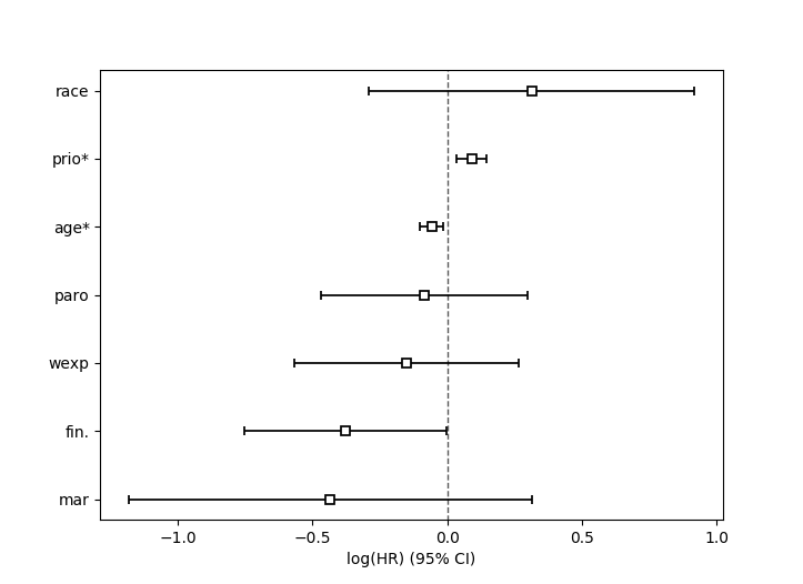
绘制系数

使用拟合模型，查看系数及其范围的另一种方法是使用plot方法。

from lifelines.datasets import load_rossi
from lifelines import CoxPHFitter

rossi = load_rossi()
cph = CoxPHFitter()
cph.fit(rossi, duration_col='week', event_col='arrest')

cph.plot()

绘制协变量变化的影响

拟合后，我们可以绘制生存曲线，当我们改变单个协变量时，保持其他所有条件不变。这对于理解协变量的影响非常有用，给定模型。为此，我们使用plot_partial_effects_on_outcome()方法，并给它感兴趣的协变量和要显示的值。

注意

在lifelines v0.25.0之前，这个方法被称为plot_covariate_groups。它已被重命名为plot_partial_effects_on_outcome（我希望这是一个更清晰的名字）。

from lifelines.datasets import load_rossi
from lifelines import CoxPHFitter

rossi = load_rossi()
cph = CoxPHFitter()
cph.fit(rossi, duration_col='week', event_col='arrest')

cph.plot_partial_effects_on_outcome(covariates='prio', values=[0, 2, 4, 6, 8, 10], cmap='coolwarm')

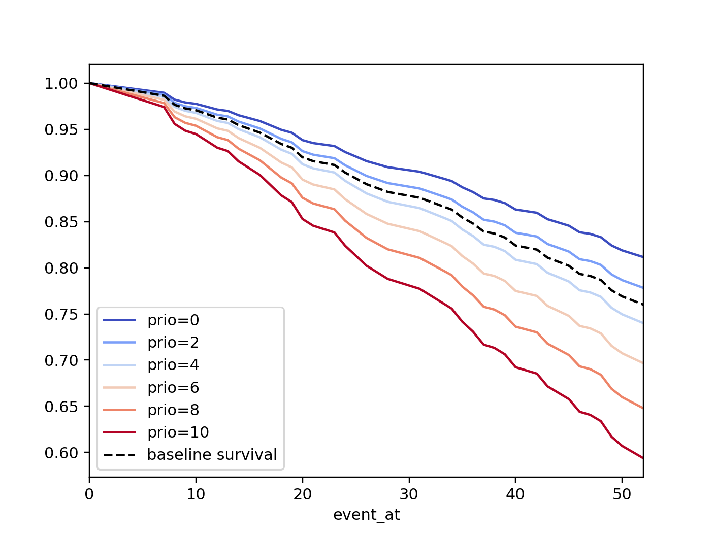
如果你的数据集中有衍生特征，例如，假设你在数据集中包含了prio和prio**2。仅仅改变year而保持year**2不变是没有意义的。你需要手动指定协变量在N维数组或列表中的取值（其中N是被改变的协变量的数量）。

rossi['prio**2'] = rossi['prio'] ** 2

cph.fit(rossi, 'week', 'arrest')

cph.plot_partial_effects_on_outcome(
    covariates=['prio', 'prio**2'],
    values=[
        [0, 0],
        [1, 1],
        [2, 4],
        [3, 9],
        [8, 64],
    ],
    cmap='coolwarm')

然而，如果你在fit中使用了formula参数，所有必要的转换将在内部自动完成。

cph.fit(rossi, 'week', 'arrest', formula="prio + I(prio**2)")

cph.plot_partial_effects_on_outcome(
    covariates=['prio'],
    values=[0, 1, 2, 3, 8],
    cmap='coolwarm')

此功能对于分析分类变量也很有用：

cph.plot_partial_effects_on_outcome(
    covariates=["a_categorical_variable"]
    values=["A", "B", ...],
    plot_baseline=False)

检查比例风险假设

为了做出正确的推断，我们应该询问我们的Cox模型是否适合我们的数据集。回想一下，在使用Cox模型时，我们隐含地应用了比例风险假设。我们应该问，我们的数据集是否遵守这一假设？

CoxPHFitter 有一个 check_assumptions() 方法，可以输出违反比例风险假设的情况。有关如何修复违反情况的教程，请参阅 Testing the Proportional Hazard Assumptions。建议寻找方法来分层某一列（参见下面的文档），或使用时间变化模型。

注意

只有在你的目标是推断或相关性时，才需要检查这样的假设。也就是说，你希望了解协变量对生存时间和结果的影响。如果你的目标是预测，检查模型假设就不那么重要了，因为你的目标是最大化准确性指标，而不是了解模型如何做出预测。

分层

有时一个或多个协变量可能不满足比例风险假设。在这种情况下，我们可以允许协变量仍然包含在模型中，而不估计其效果。这被称为分层。从高层次来看，可以将其视为将数据集分割成m个较小的数据集，按分层协变量的唯一值进行分区。每个数据集都有自己的基线风险（模型的非参数部分），但它们都共享回归参数（模型的参数部分）。由于每个数据集内的协变量是相同的，因此对于分层的协变量没有回归参数，因此它们不会出现在输出中。然而，在baseline_cumulative_hazard_下会有m个基线风险。

要指定用于分层的变量，我们在调用fit()时定义它们：

from lifelines.datasets import load_rossi
from lifelines import CoxPHFitter
rossi = load_rossi()

cph = CoxPHFitter()
cph.fit(rossi, 'week', event_col='arrest', strata=['wexp'])
cph.print_summary()

"""
<lifelines.CoxPHFitter: fitted with 432 total observations, 318 right-censored observations>
             duration col = 'week'
                event col = 'arrest'
                   strata = ['wexp']
      baseline estimation = breslow
   number of observations = 432
number of events observed = 114
   partial log-likelihood = -580.89
         time fit was run = 2020-08-09 21:25:37 UTC

---
            coef  exp(coef)   se(coef)   coef lower 95%   coef upper 95%  exp(coef) lower 95%  exp(coef) upper 95%
covariate
fin        -0.38       0.68       0.19            -0.76            -0.01                 0.47                 0.99
age        -0.06       0.94       0.02            -0.10            -0.01                 0.90                 0.99
race        0.31       1.36       0.31            -0.30             0.91                 0.74                 2.49
mar        -0.45       0.64       0.38            -1.20             0.29                 0.30                 1.34
paro       -0.08       0.92       0.20            -0.47             0.30                 0.63                 1.35
prio        0.09       1.09       0.03             0.03             0.15                 1.04                 1.16
              z      p   -log2(p)
covariate
fin       -1.99   0.05       4.42
age       -2.64   0.01       6.91
race       1.00   0.32       1.65
mar       -1.19   0.23       2.09
paro      -0.42   0.67       0.57
prio       3.16 <0.005       9.33
---
Concordance = 0.61
Partial AIC = 1173.77
log-likelihood ratio test = 23.77 on 6 df
-log2(p) of ll-ratio test = 10.77

"""

cph.baseline_survival_.shape
# (49, 2)
cph.baseline_cumulative_hazard_.plot(drawstyle="steps")

权重与稳健误差

观测值也可以带有权重。这些权重可能是表示某些常见观测值的整数值，也可能是表示某些抽样权重的浮点值（例如：逆概率权重）。在fit()方法中，有一个kwarg用于指定DataFrame中的哪一列应作为权重，例如：CoxPHFitter(df, 'T', 'E', weights_col='weights')。

在使用抽样权重时，正确的方法是同时改变标准误差的计算。这是通过在fit()中打开robust标志来实现的。在内部，CoxPHFitter将使用三明治估计器来计算误差。

import pandas as pd
from lifelines import CoxPHFitter

df = pd.DataFrame({
    'T': [5, 3, 9, 8, 7, 4, 4, 3, 2, 5, 6, 7],
    'E': [1, 1, 1, 1, 1, 1, 0, 0, 1, 1, 1, 0],
    'weights': [1.1, 0.5, 2.0, 1.6, 1.2, 4.3, 1.4, 4.5, 3.0, 3.2, 0.4, 6.2],
    'month': [10, 3, 9, 8, 7, 4, 4, 3, 2, 5, 6, 7],
    'age': [4, 3, 9, 8, 7, 4, 4, 3, 2, 5, 6, 7],
})

cph = CoxPHFitter()
cph.fit(df, 'T', 'E', weights_col='weights', robust=True)
cph.print_summary()

查看更多示例，请访问在Cox模型中为观察值添加权重。

集群与相关性

您的数据集可能具有的另一个属性是相关主题的组。这可能是由以下原因引起的：

• 一个个体有多个发生，因此在数据集中出现多次。

• 共享某些共同属性的主题，如同一个家庭的成员或根据倾向得分匹配的成员。

我们将这些分组主题称为“集群”，并假设它们由DataFrame中的某列指定（如下例所示）。当使用集群时，模型的点估计不会改变，但标准误差会增加。对此的一个直观论点是，100个个体上的100次观测比10个个体（或集群）上的100次观测提供更多的信息。

from lifelines import CoxPHFitter

df = pd.DataFrame({
    'T': [5, 3, 9, 8, 7, 4, 4, 3, 2, 5, 6, 7],
    'E': [1, 1, 1, 1, 1, 1, 0, 0, 1, 1, 1, 0],
    'month': [10, 3, 9, 8, 7, 4, 4, 3, 2, 5, 6, 7],
    'age': [4, 3, 9, 8, 7, 4, 4, 3, 2, 5, 6, 7],
    'id': [1, 1, 1, 1, 2, 3, 3, 4, 4, 5, 6, 7]
})

cph = CoxPHFitter()
cph.fit(df, 'T', 'E', cluster_col='id')
cph.print_summary()

更多示例，请参见Correlations between subjects in a Cox model。

残差

在拟合Cox模型后，我们可以回顾并计算重要的模型残差。这些残差可以告诉我们未捕捉到的非线性、比例风险假设的违反情况，并帮助我们回答其他有用的建模问题。参见使用残差评估Cox模型拟合。

使用参数模型建模基线风险和生存

通常，Cox模型是半参数的，这意味着其基线风险\(h_0(t)\)没有参数形式。这是lifelines的默认设置。然而，有时生成参数基线是有价值的。参数基线使生存预测更有效，有助于更好地理解基线行为，并允许插值/外推。

在lifelines中，可以选择使用1) 三次样条或2) 分段常数风险来拟合参数基线。三次样条非常灵活，几乎可以像非参数方法一样捕捉到基础数据，并且效率更高。

from lifelines.datasets import load_rossi
from lifelines import CoxPHFitter

rossi = load_rossi()

cph_spline = CoxPHFitter(baseline_estimation_method="spline", n_baseline_knots=5)
cph_spline.fit(rossi, 'week', event_col='arrest')

要访问基线风险和基线生存率，可以分别使用baseline_hazard_和baseline_survival_。参数模型的一个优点是我们可以插值基线生存率/风险，参见baseline_hazard_at_times()和baseline_survival_at_times()。

下面我们比较非参数和完全参数的基线生存率：

cph_semi = CoxPHFitter().fit(rossi, 'week', event_col='arrest')
cph_piecewise = CoxPHFitter(baseline_estimation_method="piecewise", breakpoints=[20, 35]).fit(rossi, 'week', event_col='arrest')

bch_key = "baseline cumulative hazard"

ax = cph_spline.baseline_cumulative_hazard_[bch_key].plot(label="spline")
cph_semi.baseline_cumulative_hazard_[bch_key].plot(ax=ax, drawstyle="steps-post", label="semi")
cph_piecewise.baseline_cumulative_hazard_[bch_key].plot(ax=ax, label="piecewise[20,35]")
plt.legend()

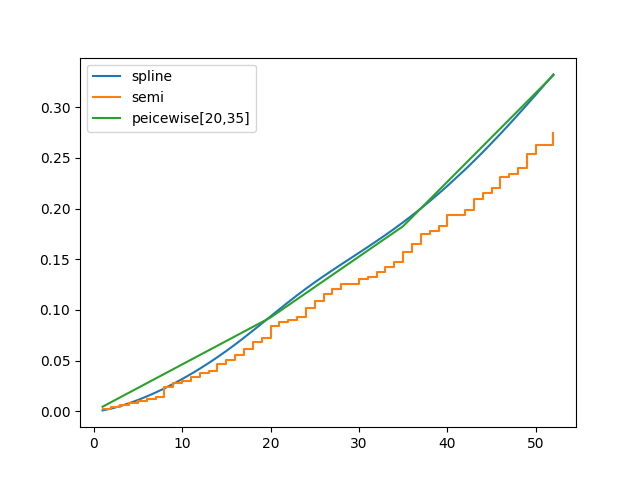
使用样条与非参数方法建模基线生存。

lifelines’ 样条Cox模型也可以使用几乎所有非参数选项，包括：strata、penalizer、timeline、formula等。

参数生存模型

我们在上一节结束时讨论了一个完全参数化的Cox模型，但还有许多其他参数化模型需要考虑。下面我们将从最常见的AFT模型开始，逐一介绍这些模型。

加速失效时间模型

假设我们有两个群体，A和B，它们有不同的生存函数，\(S_A(t)\) 和 \(S_B(t)\)，并且它们通过某种加速故障率，\(\lambda\) 相关联：

\[S_A(t) = S_B\left(\frac{t}{\lambda}\right)\]

这可以解释为减慢或加快沿着生存函数的移动。一个经典的例子是，狗的衰老速度是人类的7倍，即\(\lambda = \frac{1}{7}\)。这个模型还有其他一些很好的特性：群体B的平均生存时间是群体A的平均生存时间的\({\lambda}\)倍。同样适用于中位生存时间。

更一般地，我们可以将\(\lambda\)建模为可用协变量的函数，即：

\[\begin{split}S_A(t) = S_B\left(\frac{t}{\lambda(x)}\right)\\ \lambda(x) = \exp\left(b_0 + \sum_{i=1}^n b_i x_i \right)\end{split}\]

该模型可以根据受试者的协变量加速或减速失效时间。另一个优点是系数的解释非常容易：\(x_i\) 的单位增加意味着平均/中位生存时间变化了 \(\exp(b_i)\) 倍。

注意

关于解释的一个重要注意事项：假设\(b_i\)为正，那么因子\(\exp(b_i)\)大于1，这将减缓事件时间，因为我们用因子除以时间⇿增加平均/中位生存时间。因此，这将是一个保护效应。同样，负的\(b_i\)将加速事件时间⇿减少平均/中位生存时间。这种解释与Cox模型中符号如何影响事件时间的方式相反！这是标准的生存分析惯例。

接下来，我们为生存函数\(S(t)\)选择一个参数形式。最常见的是威布尔形式。因此，如果我们假设上述关系和威布尔形式，我们的风险函数就很容易写出来：

\[H(t; x) = \left( \frac{t}{\lambda(x)} \right)^\rho\]

我们称这些为加速失效时间模型，通常简称为AFT模型。使用lifelines，我们可以拟合这个模型（以及未知的\(\rho\)参数）。

威布尔AFT模型

Weibull AFT 模型在 WeibullAFTFitter 下实现。该类的 API 与 lifelines 中的其他回归模型类似。拟合后，可以使用 params_ 或 summary 访问系数，或者使用 print_summary() 打印。

from lifelines import WeibullAFTFitter
from lifelines.datasets import load_rossi

rossi = load_rossi()

aft = WeibullAFTFitter()
aft.fit(rossi, duration_col='week', event_col='arrest')

aft.print_summary(3)  # access the results using aft.summary

"""
<lifelines.WeibullAFTFitter: fitted with 432 observations, 318 censored>
      duration col = 'week'
         event col = 'arrest'
number of subjects = 432
  number of events = 114
    log-likelihood = -679.917
  time fit was run = 2019-02-20 17:47:19 UTC

---
                     coef  exp(coef)  se(coef)      z       p  -log2(p)  lower 0.95  upper 0.95
lambda_ fin         0.272      1.313     0.138  1.973   0.049     4.365       0.002       0.543
        age         0.041      1.042     0.016  2.544   0.011     6.512       0.009       0.072
        race       -0.225      0.799     0.220 -1.021   0.307     1.703      -0.656       0.207
        wexp        0.107      1.112     0.152  0.703   0.482     1.053      -0.190       0.404
        mar         0.311      1.365     0.273  1.139   0.255     1.973      -0.224       0.847
        paro        0.059      1.061     0.140  0.421   0.674     0.570      -0.215       0.333
        prio       -0.066      0.936     0.021 -3.143   0.002     9.224      -0.107      -0.025
        Intercept  3.990     54.062     0.419  9.521 <0.0005    68.979       3.169       4.812
rho_    Intercept  0.339      1.404     0.089  3.809 <0.0005    12.808       0.165       0.514
---
Concordance = 0.640
AIC = 1377.833
log-likelihood ratio test = 33.416 on 7 df
-log2(p) of ll-ratio test = 15.462
"""

从上面我们可以看到，prio，即之前的监禁次数，有一个很大的负系数。这意味着每次额外的监禁会使受试者的平均/中位生存时间改变\(\exp(-0.066) = 0.936\)，大约减少了7%的平均/中位生存时间。什么是平均/中位生存时间？

print(aft.median_survival_time_)
print(aft.mean_survival_time_)

# 100.325
# 118.67

上表中的rho_    _intercept行是什么意思？在内部，我们对rho_参数的对数进行建模，因此\(\rho\)的值是该值的指数，所以在上述情况下是\(\hat{\rho} = \exp0.339 = 1.404\)。这引出了下一个点——使用协变量对\(\rho\)进行建模：

建模辅助参数

在上述模型中，我们将参数\(\rho\)保留为单一未知数。我们也可以选择对这个参数进行建模。为什么我们可能想要这样做呢？它可以帮助在生存预测中允许\(\rho\)参数的异质性。该模型不再是AFT模型，但我们仍然可以通过查看其结果图来恢复和理解改变协变量的影响（见下文部分）。为了对\(\rho\)进行建模，我们在调用fit()时使用ancillary关键字参数。有四个有效的选项：

1. False 或 None：明确不建模 rho_ 参数（除了其截距）。

2. 一个Pandas DataFrame。此选项将使用Pandas DataFrame中的列作为回归中的协变量，用于rho_。这个DataFrame可以等于或用于建模lambda_的原始数据集的子集，或者它可以是一个完全不同的数据集。

3. True。传入True将在内部重用用于建模lambda_的数据集。

4. 一个类似R的公式。

aft = WeibullAFTFitter()

aft.fit(rossi, duration_col='week', event_col='arrest', ancillary=False)
# identical to aft.fit(rossi, duration_col='week', event_col='arrest', ancillary=None)


aft.fit(rossi, duration_col='week', event_col='arrest', ancillary=some_df)


aft.fit(rossi, duration_col='week', event_col='arrest', ancillary=True)
# identical to aft.fit(rossi, duration_col='week', event_col='arrest', ancillary=rossi)
# identical to aft.fit(rossi, duration_col='week', event_col='arrest', ancillary="fin + age + race + wexp + mar + paro + prio")

aft.print_summary()

"""
<lifelines.WeibullAFTFitter: fitted with 432 observations, 318 censored>
      duration col = 'week'
         event col = 'arrest'
number of subjects = 432
  number of events = 114
    log-likelihood = -669.40
  time fit was run = 2019-02-20 17:42:55 UTC

---
                    coef  exp(coef)  se(coef)     z      p  -log2(p)  lower 0.95  upper 0.95
lambda_ fin         0.24       1.28      0.15  1.60   0.11      3.18       -0.06        0.55
        age         0.10       1.10      0.03  3.43 <0.005     10.69        0.04        0.16
        race        0.07       1.07      0.19  0.36   0.72      0.48       -0.30        0.44
        wexp       -0.34       0.71      0.15 -2.22   0.03      5.26       -0.64       -0.04
        mar         0.26       1.30      0.30  0.86   0.39      1.35       -0.33        0.85
        paro        0.09       1.10      0.15  0.61   0.54      0.88       -0.21        0.39
        prio       -0.08       0.92      0.02 -4.24 <0.005     15.46       -0.12       -0.04
        Intercept  2.68      14.65      0.60  4.50 <0.005     17.14        1.51        3.85
rho_    fin        -0.01       0.99      0.15 -0.09   0.92      0.11       -0.31        0.29
        age        -0.05       0.95      0.02 -3.10 <0.005      9.01       -0.08       -0.02
        race       -0.46       0.63      0.25 -1.79   0.07      3.77       -0.95        0.04
        wexp        0.56       1.74      0.17  3.32 <0.005     10.13        0.23        0.88
        mar         0.10       1.10      0.27  0.36   0.72      0.47       -0.44        0.63
        paro        0.02       1.02      0.16  0.12   0.90      0.15       -0.29        0.33
        prio        0.03       1.03      0.02  1.44   0.15      2.73       -0.01        0.08
        Intercept  1.48       4.41      0.41  3.60 <0.005     11.62        0.68        2.29
---
Concordance = 0.63
Log-likelihood ratio test = 54.45 on 14 df, -log2(p)=19.83
"""

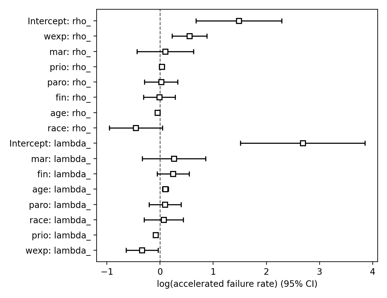
绘图

绘图API与CoxPHFitter中的相同。我们可以在森林图中查看所有协变量：

from matplotlib import pyplot as plt

wft = WeibullAFTFitter().fit(rossi, 'week', 'arrest', ancillary=True)
wft.plot()

我们可以通过绘制变量变化的结果（即生存率）来观察模型中变量的影响。这是通过使用plot_partial_effects_on_outcome()来完成的，这也是观察建模rho_与保持其固定效果的好时机。下面我们将威布尔模型两次拟合到相同的数据集，但在第一个模型中我们建模rho_，而在第二个模型中我们没有。当我们改变prio（即先前逮捕的次数）并观察生存率如何变化时。

注意

在lifelines v0.25.0之前，这个方法曾经被称为plot_covariate_group。它已被重命名为plot_partial_effects_on_outcome（我希望这是一个更清晰的名字）。

fig, ax = plt.subplots(nrows=1, ncols=2, figsize=(10, 4))

times = np.arange(0, 100)
wft_model_rho = WeibullAFTFitter().fit(rossi, 'week', 'arrest', ancillary=True, timeline=times)
wft_model_rho.plot_partial_effects_on_outcome('prio', range(0, 16, 3), cmap='coolwarm', ax=ax[0])
ax[0].set_title("Modelling rho_")

wft_not_model_rho = WeibullAFTFitter().fit(rossi, 'week', 'arrest', ancillary=False, timeline=times)
wft_not_model_rho.plot_partial_effects_on_outcome('prio', range(0, 16, 3), cmap='coolwarm', ax=ax[1])
ax[1].set_title("Not modelling rho_");

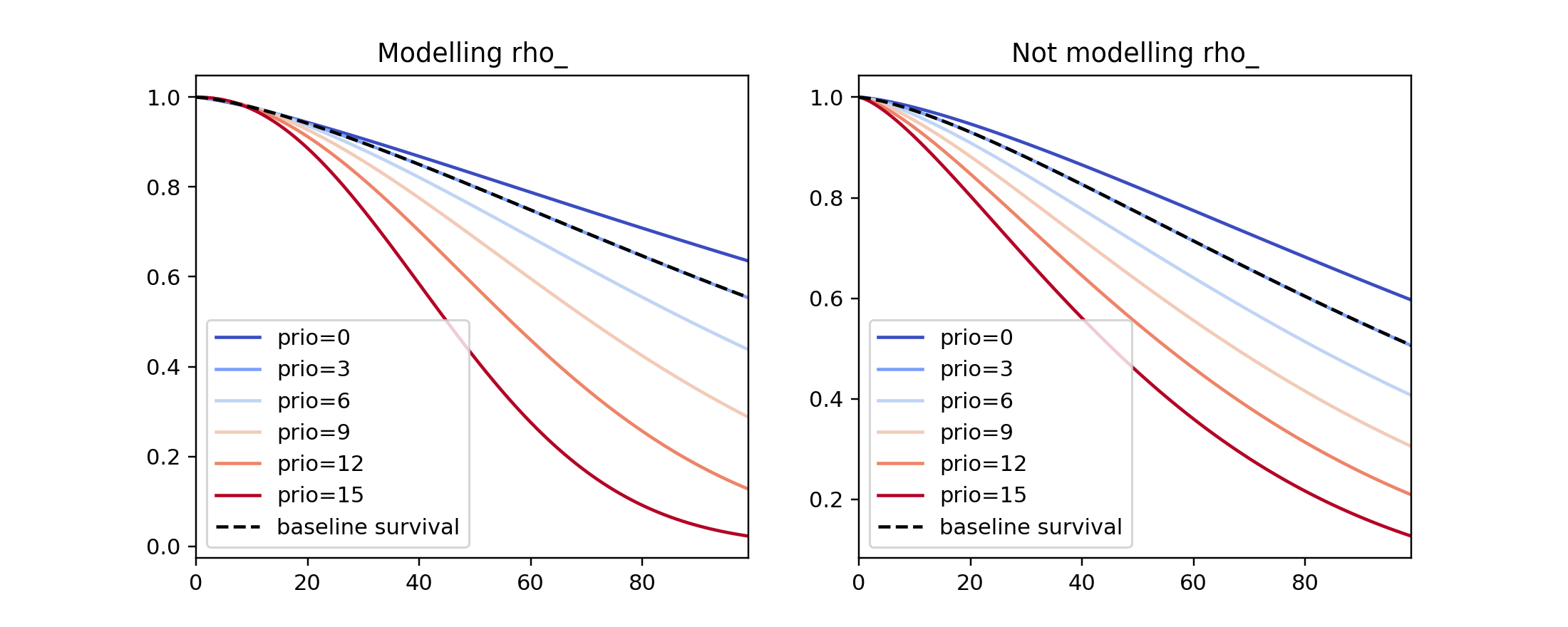
将这些生存函数并排比较，我们可以看到建模rho_会产生一组更灵活（多样化）的生存函数。

fig, ax = plt.subplots(nrows=1, ncols=1, figsize=(7, 4))

# modeling rho == solid line
wft_model_rho.plot_partial_effects_on_outcome('prio', range(0, 16, 5), cmap='coolwarm', ax=ax, lw=2, plot_baseline=False)

# not modeling rho == dashed line
wft_not_model_rho.plot_partial_effects_on_outcome('prio', range(0, 16, 5), cmap='coolwarm', ax=ax, ls='--', lw=2, plot_baseline=False)

ax.get_legend().remove()

您可以在plot_partial_effects_on_outcome()的文档中阅读更多内容并查看其他示例。

预测

给定一个新对象，我们想询问他们未来的生存情况。他们何时可能经历该事件？他们的生存函数是什么样的？WeibullAFTFitter能够回答这些问题。如果我们已经对辅助协变量进行了建模，我们也需要包括这些协变量：

X = rossi.loc[:10]

aft.predict_cumulative_hazard(X, ancillary=X)
aft.predict_survival_function(X, ancillary=X)
aft.predict_median(X, ancillary=X)
aft.predict_percentile(X, p=0.9, ancillary=X)
aft.predict_expectation(X, ancillary=X)

有两个超参数可以用来获得更好的测试分数。这些是在调用WeibullAFTFitter时的penalizer和l1_ratio。penalizer类似于scikit-learn的ElasticNet模型，参见他们的文档。（然而，lifelines也会接受一个数组用于每个变量的自定义惩罚值，参见上面的Cox文档）

aft_with_elastic_penalty = WeibullAFTFitter(penalizer=1e-4, l1_ratio=1.0)
aft_with_elastic_penalty.fit(rossi, 'week', 'arrest')
aft_with_elastic_penalty.predict_median(rossi)

aft_with_elastic_penalty.print_summary(columns=['coef', 'exp(coef)'])

"""
<lifelines.WeibullAFTFitter: fitted with 432 total observations, 318 right-censored observations>
             duration col = 'week'
                event col = 'arrest'
                penalizer = 0.0001
   number of observations = 432
number of events observed = 114
           log-likelihood = -679.97
         time fit was run = 2020-08-09 15:04:35 UTC

---
                    coef  exp(coef)
param   covariate
lambda_ age         0.04       1.04
        fin         0.27       1.31
        mar         0.31       1.36
        paro        0.06       1.06
        prio       -0.07       0.94
        race       -0.22       0.80
        wexp        0.11       1.11
        Intercept   3.99      54.11
rho_    Intercept   0.34       1.40
---
Concordance = 0.64
AIC = 1377.93
log-likelihood ratio test = 33.31 on 7 df
-log2(p) of ll-ratio test = 15.40

"""

对数正态和对数逻辑AFT模型

还有LogNormalAFTFitter和LogLogisticAFTFitter模型，它们不假设生存时间分布是Weibull，而是分别假设为对数正态或对数逻辑分布。它们的API与WeibullAFTFitter相同，但参数名称不同。

from lifelines import LogLogisticAFTFitter
from lifelines import LogNormalAFTFitter

llf = LogLogisticAFTFitter().fit(rossi, 'week', 'arrest')
lnf = LogNormalAFTFitter().fit(rossi, 'week', 'arrest')

更多AFT模型：CRC模型和广义伽马模型

对于一个灵活且平滑的参数模型，有GeneralizedGammaRegressionFitter。这个模型实际上是上述所有AFT模型的泛化（即其参数的特定值代表另一个模型）- 请参阅文档以了解特定参数值。然而，API略有不同，看起来更像自定义回归模型的构建方式（请参阅下一节关于自定义回归模型的内容）。

from lifelines import GeneralizedGammaRegressionFitter
from lifelines.datasets import load_rossi

df = load_rossi()
df['Intercept'] = 1.

# this will regress df against all 3 parameters
ggf = GeneralizedGammaRegressionFitter(penalizer=1.).fit(df, 'week', 'arrest')
ggf.print_summary()

# If we want fine control over the parameters <-> covariates.
# The values in the dict become can be formulas, or column names in lists:
regressors = {
    'mu_': rossi.columns.difference(['arrest', 'week']),
    'sigma_': ["age", "Intercept"],
    'lambda_': 'age + 1',
}

ggf = GeneralizedGammaRegressionFitter(penalizer=0.0001).fit(df, 'week', 'arrest', regressors=regressors)
ggf.print_summary()

同样地，有一个使用样条来建模时间的CRC模型。关于它的博客文章请参见这里。

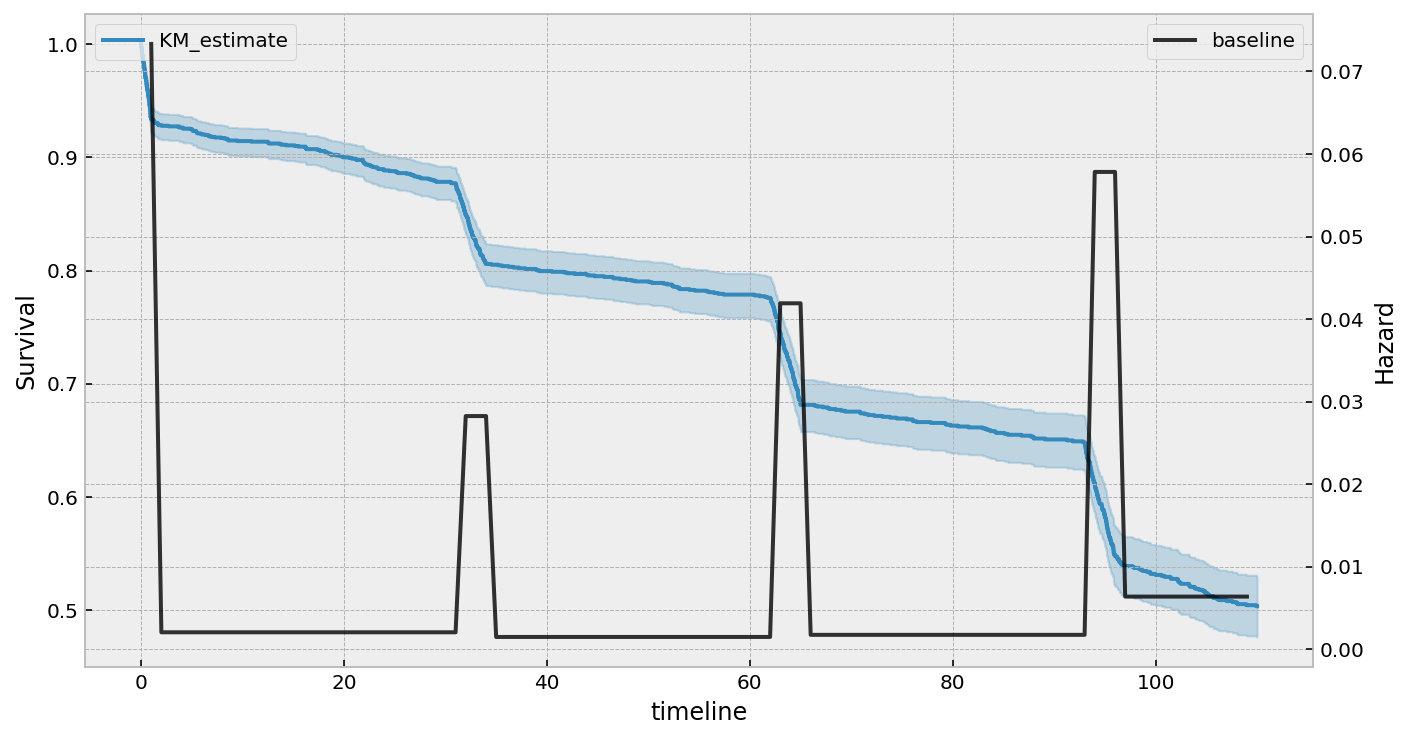
分段指数回归模型

另一类参数模型涉及对风险函数进行更灵活的建模。PiecewiseExponentialRegressionFitter 可以建模风险中的跳跃（例如：一年级、二年级、三年级和四年级学生“继续留校生存率”的差异），以及跳跃之间的恒定值。能够指定这些跳跃发生的时间（称为断点），为建模者提供了极大的灵活性。一个涉及客户流失的示例应用可以在本notebook中找到。

参数模型的AIC和模型选择

通常，你并不知道先验应该使用哪个参数模型。每个模型都有一些内置的假设（在lifelines中尚未实现），但一个快速有效的方法是比较每个拟合模型的AICs。（在这种情况下，每个模型的参数数量相同，所以实际上这是在比较对数似然）。AIC最小的模型在自由度最小的情况下对数据的拟合效果最好。

from lifelines import LogLogisticAFTFitter, WeibullAFTFitter, LogNormalAFTFitter
from lifelines.datasets import load_rossi

rossi = load_rossi()

llf = LogLogisticAFTFitter().fit(rossi, 'week', 'arrest')
lnf = LogNormalAFTFitter().fit(rossi, 'week', 'arrest')
wf = WeibullAFTFitter().fit(rossi, 'week', 'arrest')

print(llf.AIC_)  # 1377.877
print(lnf.AIC_)  # 1384.469
print(wf.AIC_)   # 1377.833, slightly the best model.


# with some heterogeneity in the ancillary parameters
ancillary = rossi[['prio']]
llf = LogLogisticAFTFitter().fit(rossi, 'week', 'arrest', ancillary=ancillary)
lnf = LogNormalAFTFitter().fit(rossi, 'week', 'arrest', ancillary=ancillary)
wf = WeibullAFTFitter().fit(rossi, 'week', 'arrest', ancillary=ancillary)

print(llf.AIC_) # 1377.89, the best model here, but not the overall best.
print(lnf.AIC_) # 1380.79
print(wf.AIC_)  # 1379.21

左、右和区间删失数据

参数模型也有处理左删失和区间删失数据的API。这些API与用于拟合右删失数据的API不同。以下是一个使用区间删失数据的示例。

from lifelines.datasets import load_diabetes

df = load_diabetes()
df['gender'] = df['gender'] == 'male'

print(df.head())
"""
   left  right  gender
1    24     27    True
2    22     22   False
3    37     39    True
4    20     20    True
5     1     16    True
"""

wf = WeibullAFTFitter().fit_interval_censoring(df, lower_bound_col='left', upper_bound_col='right')
wf.print_summary()

"""
<lifelines.WeibullAFTFitter: fitted with 731 total observations, 136 interval-censored observations>
          lower bound col = 'left'
          upper bound col = 'right'
                event col = 'E_lifelines_added'
   number of observations = 731
number of events observed = 595
           log-likelihood = -2027.20
         time fit was run = 2020-08-09 15:05:09 UTC

---
                    coef  exp(coef)   se(coef)   coef lower 95%   coef upper 95%  exp(coef) lower 95%  exp(coef) upper 95%
param   covariate
lambda_ gender      0.05       1.05       0.03            -0.01             0.10                 0.99                 1.10
        Intercept   2.91      18.32       0.02             2.86             2.95                17.53                19.14
rho_    Intercept   1.04       2.83       0.03             0.98             1.09                 2.67                 2.99
                       z      p   -log2(p)
param   covariate
lambda_ gender      1.66   0.10       3.38
        Intercept 130.15 <0.005        inf
rho_    Intercept  36.91 <0.005     988.46
---
AIC = 4060.39
log-likelihood ratio test = 2.74 on 1 df
-log2(p) of ll-ratio test = 3.35
"""

另一个使用lifelines处理区间删失数据的例子位于这里。

自定义参数回归模型

lifelines 有一个非常通用的语法来创建您自己的参数回归模型。如果您想创建自己的自定义模型，请参阅文档 自定义回归模型。

Aalen的加性模型

警告

此实现仍处于实验阶段。

Aalen的加性模型是我们可以使用的另一种回归模型。与Cox模型类似，它定义了风险率，但与Cox模型的线性模型是乘法不同，Aalen模型是加法的。具体来说：

\[h(t|x) = b_0(t) + b_1(t) x_1 + ... + b_N(t) x_N\]

推断通常不估计个体的 \(b_i(t)\)，而是估计\(\int_0^t b_i(s) \; ds\) （类似于使用NelsonAalenFitter估计风险率）。这在解释生成的图表时非常重要。

在这个练习中，我们将使用政权数据集，并包括分类变量un_continent_name（例如：亚洲、北美洲等），regime类型（例如，君主制、平民等）以及政权开始的年份start_year。用于拟合Aalen加法模型中未知系数的估计器位于AalenAdditiveFitter下。

from lifelines import AalenAdditiveFitter
from lifelines.datasets import load_dd

data = load_dd()
data.head()

国家名称	cowcode2	politycode	un_region_name	un_continent_name	ehead	leaderspellreg	民主	制度	起始年份	持续时间	观察到的
阿富汗	700	700	南亚	亚洲	穆罕默德·查希尔·沙阿	穆罕默德·查希尔·沙阿。阿富汗。1946年。1952年。君主制	非民主	君主制	1946	7	1
阿富汗	700	700	南亚	亚洲	萨达尔·穆罕默德·达乌德	萨达尔·穆罕默德·达乌德。阿富汗。1953年。1962年。文官独裁	非民主	民用词典	1953	10	1
阿富汗	700	700	南亚	亚洲	穆罕默德·查希尔·沙阿	穆罕默德·查希尔·沙阿。阿富汗。1963年。1972年。君主制	非民主	君主制	1963	10	1
阿富汗	700	700	南亚	亚洲	萨达尔·穆罕默德·达乌德	萨达尔·穆罕默德·达乌德。阿富汗。1973年。1977年。平民独裁	非民主	民用词典	1973	5	0
阿富汗	700	700	南亚	亚洲	努尔·穆罕默德·塔拉基	努尔·穆罕默德·塔拉基。阿富汗。1978年。1978年。平民独裁	非民主	民用词典	1978	1	0

我们还包含了coef_penalizer选项。在估计过程中，每一步都会计算一个线性回归。通常，回归可能会不稳定（由于高共线性或小样本量）——添加一个惩罚项可以控制稳定性。我建议始终从一个小的惩罚项开始——如果估计结果仍然显得不稳定，尝试增加它。

aaf = AalenAdditiveFitter(coef_penalizer=1.0, fit_intercept=False)

AalenAdditiveFitter 的一个实例包含一个 fit() 方法，该方法对系数进行推断。此方法接受一个 pandas DataFrame：每一行代表一个个体，列是协变量和两个单独的列：一个 duration 列和一个布尔 event occurred 列（其中 event occurred 指的是感兴趣的事件 - 在这种情况下是从政府中驱逐）

data['T'] = data['duration']
data['E'] = data['observed']

aaf.fit(data, 'T', event_col='E', formula='un_continent_name + regime + start_year')

拟合后，实例会暴露一个cumulative_hazards_ DataFrame，其中包含\(\int_0^t b_i(s) \; ds\)的估计值：

aaf.cumulative_hazards_.head()

基线	un_continent_name[T.Americas]	un_continent_name[T.亚洲]	un_continent_name[T.欧洲]	un_continent_name[T.大洋洲]	政权[T.军事独裁]	regime[T.Mixed Dem]	regime[T.Monarchy]	政权[T.议会民主]	政权[T.总统民主]	起始年份
-0.03447	-0.03173	0.06216	0.2058	-0.009559	0.07611	0.08729	-0.1362	0.04885	0.1285	0.000092
0.14278	-0.02496	0.11122	0.2083	-0.079042	0.11704	0.36254	-0.2293	0.17103	0.1238	0.000044
0.30153	-0.07212	0.10929	0.1614	0.063030	0.16553	0.68693	-0.2738	0.33300	0.1499	0.000004
0.37969	0.06853	0.15162	0.2609	0.185569	0.22695	0.95016	-0.2961	0.37351	0.4311	-0.000032
0.36749	0.20201	0.21252	0.2429	0.188740	0.25127	1.15132	-0.3926	0.54952	0.7593	-0.000000

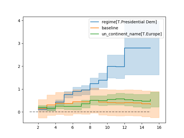
AalenAdditiveFitter 也有内置的绘图功能：

aaf.plot(columns=['regime[T.Presidential Dem]', 'Intercept', 'un_continent_name[T.Europe]'], iloc=slice(1,15))

如果我们将其用于尚未见过的数据，即预测，回归将是最有趣的！我们可以使用我们所学到的知识来预测个体的风险率、生存函数和中位生存时间。我们使用的数据集截至2008年，所以让我们使用这些数据来预测加拿大前总理斯蒂芬·哈珀的任期。

ix = (data['ctryname'] == 'Canada') & (data['start_year'] == 2006)
harper = data.loc[ix]
print("Harper's unique data point:")
print(harper)

Harper's unique data point:
     baseline  un_continent_name[T.Americas]  un_continent_name[T.Asia] ...  start_year  T  E
268       1.0                            1.0                        0.0 ...      2006.0  3  0

ax = plt.subplot(2,1,1)
aaf.predict_cumulative_hazard(harper).plot(ax=ax)

ax = plt.subplot(2,1,2)
aaf.predict_survival_function(harper).plot(ax=ax);

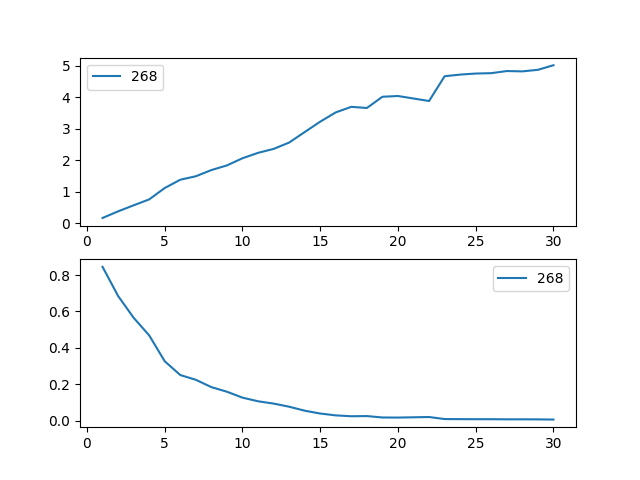
注意

由于模型的性质，个体的估计生存函数可能会增加。这是Aalen加法模型的预期产物。

生存回归中的模型选择和校准

参数模型与半参数模型

上面，我们展示了两个半参数模型（Cox模型和Aalen模型），以及一系列参数模型。你应该选择哪一个？它们各自的优缺点是什么？我建议阅读以下两个StackExchange的答案，以更好地了解专家们的看法：

1. 在生存分析中，为什么我们使用半参数模型（Cox比例风险模型）而不是完全参数模型？

2. 在生存分析中，我们何时应该使用完全参数模型而不是半参数模型？

基于残差的模型选择

章节Testing the Proportional Hazard Assumptions和Assessing Cox model fit using residuals可能对更好地建模您的数据有用。

注意

正在进行工作以将残差方法扩展到所有回归模型。敬请期待。

基于预测能力和拟合度的模型选择

如果存在截尾数据，使用均方误差或平均绝对损失等损失函数是不合适的。这是因为截尾值与预测值之间的差异可能是由于预测不佳或截尾造成的。下面我们介绍衡量预测性能的替代方法。

对数似然

在作者看来，衡量预测性能的最佳方法是评估样本外数据的对数似然。对数似然正确处理任何类型的截尾，并且正是我们在模型训练中最大化的内容。样本内对数似然可在任何回归模型的log_likelihood_下获得。对于样本外数据，可以使用score()方法（所有回归模型都可用）。这将返回样本外对数似然的平均评估。我们希望最大化这个值。

from lifelines import CoxPHFitter
from lifelines.datasets import load_rossi

rossi = load_rossi().sample(frac=1.0, random_state=25)  # ensures the reproducibility of the example
train_rossi = rossi.iloc[:400]
test_rossi = rossi.iloc[400:]

cph_l1 = CoxPHFitter(penalizer=0.1, l1_ratio=1.).fit(train_rossi, 'week', 'arrest')
cph_l2 = CoxPHFitter(penalizer=0.1, l1_ratio=0.).fit(train_rossi, 'week', 'arrest')

print(cph_l1.score(test_rossi))
print(cph_l2.score(test_rossi))  # higher is better

赤池信息准则 (AIC)

对于样本内验证，AIC 是一个很好的比较模型的指标，因为它依赖于对数似然。对于参数模型，可以在 AIC_ 下找到它，而对于 Cox 模型，可以在 AIC_partial_ 下找到它（因为 Cox 模型最大化的是部分对数似然，所以不能可靠地与参数模型的 AIC 进行比较。）

from lifelines import CoxPHFitter
from lifelines.datasets import load_rossi

rossi = load_rossi()

cph_l2 = CoxPHFitter(penalizer=0.1, l1_ratio=0.).fit(rossi, 'week', 'arrest')
cph_l1 = CoxPHFitter(penalizer=0.1, l1_ratio=1.).fit(rossi, 'week', 'arrest')

print(cph_l2.AIC_partial_) # lower is better
print(cph_l1.AIC_partial_)

一致性指数

另一个对审查敏感的指标是concordance-index，也称为c-index。该指标评估预测时间的排序准确性。它实际上是AUC（另一种常见的损失函数）的泛化，并且解释方式类似：

• 0.5 是随机预测的预期结果，

• 1.0 表示完全一致，

• 0.0 表示完全的反一致性（将预测值乘以 -1 得到 1.0）

Here 是新用户了解c-index的绝佳介绍和描述。

拟合的生存模型通常具有0.55到0.75之间的一致性指数（这可能看起来不太好，但即使是一个完美的模型也有很多噪声，这使得高分变得不可能）。在lifelines中，拟合模型的一致性指数出现在score()的输出中，也可以在concordance_index_属性下找到。通常，该度量在lifelines中通过lifelines.utils.concordance_index()实现，并接受实际时间（以及任何被审查的受试者）和预测时间。

from lifelines import CoxPHFitter
from lifelines.datasets import load_rossi

rossi = load_rossi()

cph = CoxPHFitter()
cph.fit(rossi, duration_col="week", event_col="arrest")

# fours ways to view the c-index:
# method one
cph.print_summary()

# method two
print(cph.concordance_index_)

# method three
print(cph.score(rossi, scoring_method="concordance_index"))

# method four
from lifelines.utils import concordance_index
print(concordance_index(rossi['week'], -cph.predict_partial_hazard(rossi), rossi['arrest']))

注意

记住，一致性评分评估的是受试者事件时间的相对排名。因此，它是尺度和位移不变的（即你可以乘以一个正常数，或加上一个常数，排名不会改变）。一个为一致性指数最大化的模型不一定能给出好的预测时间，但会给出好的预测排名。

交叉验证

lifelines 在 lifelines.utils.k_fold_cross_validation() 下实现了 k 折交叉验证。该函数接受一个回归拟合器的实例（可以是 CoxPHFitter 或 AalenAdditiveFitter）、一个数据集，以及 k（要执行的折数，默认为 5）。在每一折中，它将数据分为训练集和测试集，在训练集上拟合自身，并在测试集上评估自身（默认使用一致性度量）。

from lifelines import CoxPHFitter
from lifelines.datasets import load_regression_dataset
from lifelines.utils import k_fold_cross_validation

regression_dataset = load_regression_dataset()
cph = CoxPHFitter()
scores = k_fold_cross_validation(cph, regression_dataset, 'T', event_col='E', k=3)
print(scores)
#[-2.9896, -3.08810, -3.02747]

scores = k_fold_cross_validation(cph, regression_dataset, 'T', event_col='E', k=3, scoring_method="concordance_index")
print(scores)
# [0.5449, 0.5587, 0.6179]

此外，lifelines 还提供了与 scikit learn 兼容的包装器，使得交叉验证和网格搜索更加容易。

模型概率校准

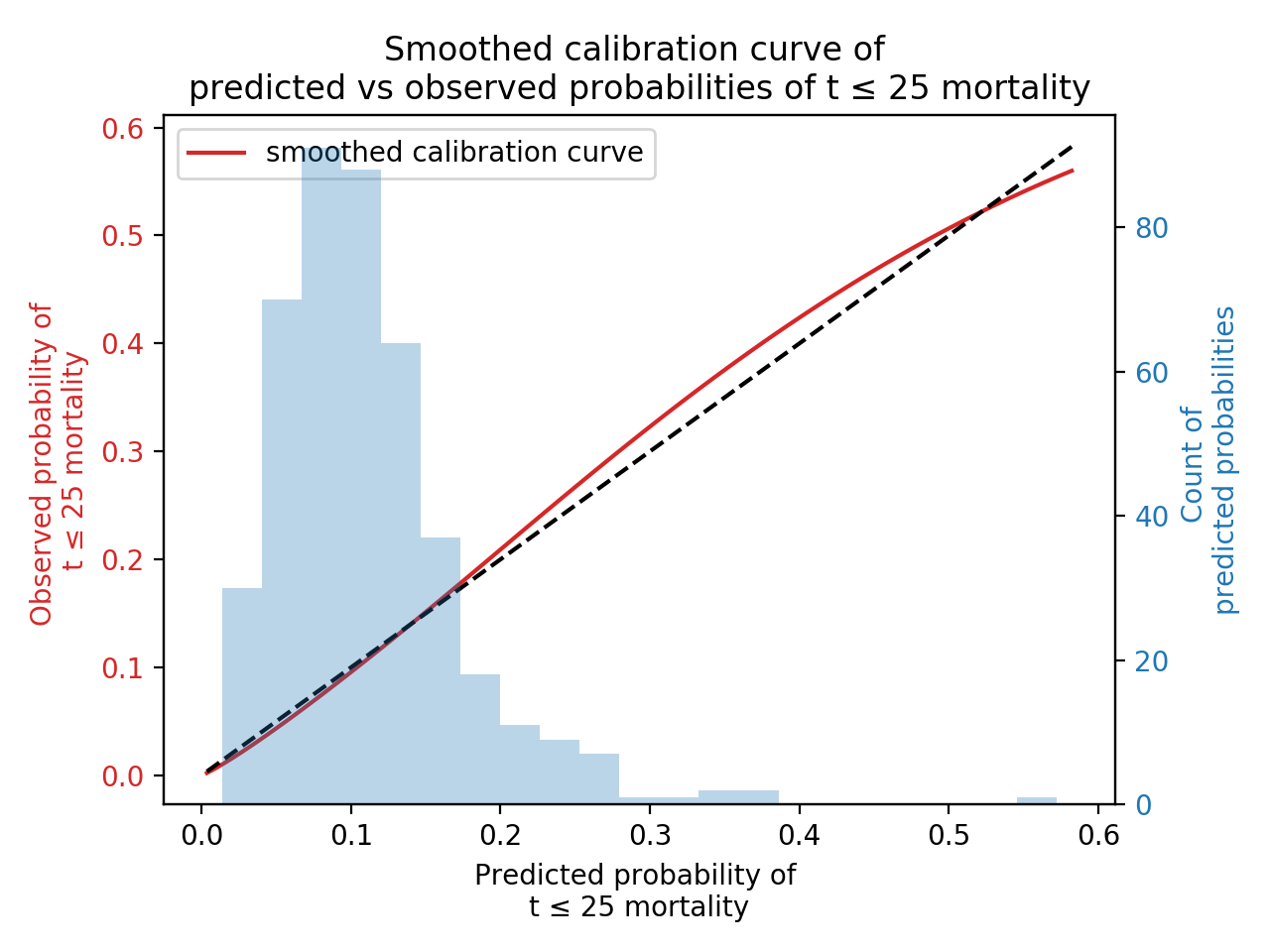
在lifelines v0.24.11版本中新增了survival_probability_calibration()函数，用于根据观察到的事件频率来测量拟合的生存模型。我们遵循P. Austin及其同事在“生存模型的图形校准曲线和综合校准指数（ICI）”中的建议，使用灵活的样条回归模型创建平滑的校准曲线（这避免了传统方法中对连续值概率进行分箱的问题，并处理了删失数据）。

from lifelines import CoxPHFitter
from lifelines.datasets import load_rossi
from lifelines.calibration import survival_probability_calibration

regression_dataset = load_rossi()
cph = CoxPHFitter(baseline_estimation_method="spline", n_baseline_knots=3)
cph.fit(rossi, "week", "arrest")


survival_probability_calibration(cph, rossi, t0=25)

对删失对象的预测

一个常见的用例是预测被审查对象的事件时间。这很容易做到，但我们首先需要计算一个重要的条件概率。设\(T\)为某个对象的（随机）事件时间，\(S(t)≔P(T > t)\)为其生存函数。我们感兴趣的是回答以下问题：如果我知道对象已经活过了时间:math:`s`，那么对象的新生存函数是什么？ 数学上表示为：

\[\begin{split}\begin{align*} P(T > t \;|\; T > s) &= \frac{P(T > t \;\text{and}\; T > s)}{P(T > s)} \\ &= \frac{P(T > t)}{P(T > s)} \\ &= \frac{S(t)}{S(s)} \end{align*}\end{split}\]

因此，我们将原始生存函数按时间\(s\)的生存函数进行缩放（在\(s\)之前的所有内容也应映射到1.0，因为我们处理的是概率，并且我们知道受试者在\(s\)之前是活着的）。

这是一个非常常见的计算，因此lifelines已经内置了所有这些功能。所有预测方法中的conditional_after kwarg允许您为每个主题指定\(s\)是什么。下面我们预测被审查主题的剩余寿命：

# all regression models can be used here, WeibullAFTFitter is used for illustration
wf = WeibullAFTFitter().fit(rossi, "week", "arrest")

# filter down to just censored subjects to predict remaining survival
censored_subjects = rossi.loc[~rossi['arrest'].astype(bool)]
censored_subjects_last_obs = censored_subjects['week']

# predict new survival function
wf.predict_survival_function(censored_subjects, conditional_after=censored_subjects_last_obs)

# predict median remaining life
wf.predict_median(censored_subjects, conditional_after=censored_subjects_last_obs)

注意

重要的是要记住，现在计算的是条件概率（或度量），因此如果predict_median的结果是10.5，那么整个生命周期就是10.5 + conditional_after。

注意

如果使用conditional_after来预测未删失的受试者，那么conditional_after可能应该设置为0，或者留空。