---

%matplotlib inline
%config InlineBackend.figure_format = 'retina'

from matplotlib import pyplot as plt
from lifelines import CoxPHFitter
import numpy as np
import pandas as pd
from lifelines.datasets import load_rossi

plt.style.use('bmh')

使用残差评估Cox模型拟合度（进行中）

本教程将介绍Cox模型的（众多）残差的一些常见用例。我们可以使用残差来诊断模型对数据集的拟合不佳，并改进现有模型的拟合效果。

df = load_rossi()

df['age_strata'] = pd.cut(df['age'], np.arange(0, 80, 5))
df = df.drop('age', axis=1)

cph = CoxPHFitter()
cph.fit(df, 'week', 'arrest', strata=['age_strata', 'wexp'])

<lifelines.CoxPHFitter: fitted with 432 total observations, 318 right-censored observations>

cph.print_summary()
cph.plot();

model	lifelines.CoxPHFitter
duration col	'week'
event col	'arrest'
strata	[age_strata, wexp]
baseline estimation	breslow
number of observations	432
number of events observed	114
partial log-likelihood	-434.50
time fit was run	2020-07-26 22:06:07 UTC

	coef	exp(coef)	se(coef)	coef lower 95%	coef upper 95%	exp(coef) lower 95%	exp(coef) upper 95%	z	p	-log2(p)
covariate
fin	-0.41	0.67	0.19	-0.79	-0.03	0.46	0.97	-2.10	0.04	4.82
race	0.29	1.33	0.31	-0.32	0.90	0.73	2.45	0.93	0.35	1.50
mar	-0.34	0.71	0.39	-1.10	0.42	0.33	1.52	-0.87	0.38	1.38
paro	-0.10	0.91	0.20	-0.48	0.29	0.62	1.33	-0.50	0.62	0.70
prio	0.08	1.08	0.03	0.02	0.14	1.03	1.15	2.83	<0.005	7.73

Concordance	0.57
Partial AIC	879.01
log-likelihood ratio test	13.12 on 5 df
-log2(p) of ll-ratio test	5.49

鞅残差

定义为：

\[\begin{split}\delta_i - \Lambda(T_i) \\ = \delta_i - \beta_0(T_i)\exp(\beta^T x_i)\end{split}\]

其中 \(T_i\) 是受试者 \(i\) 的总观察时间，\(\delta_i\) 表示他们是否在观察期间死亡（在 lifelines 中的 event_observed）。

来自 [1]:

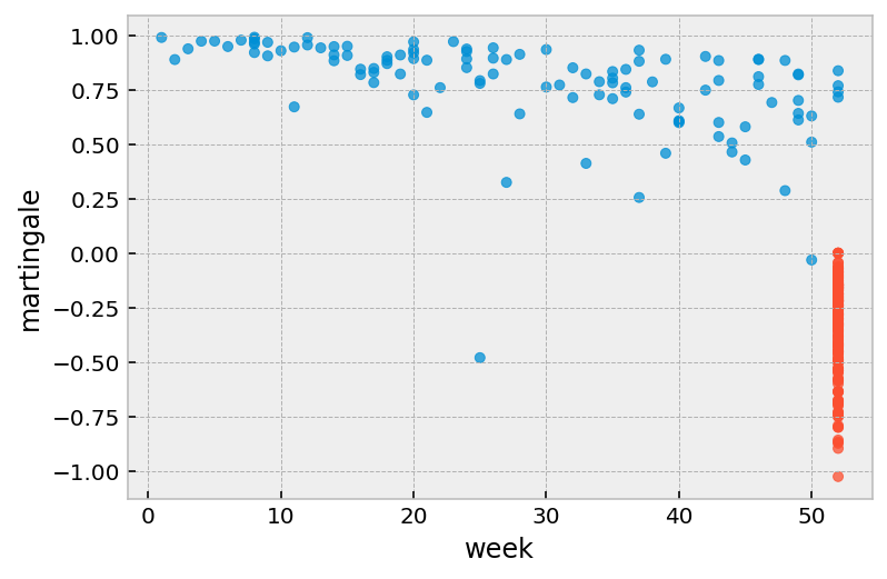
Martingale残差对于未删失的观测值取值为\([1,−\inf]\)，对于删失的观测值取值为\([0,−\inf]\)。Martingale残差可用于评估特定协变量的真实函数形式（Thernau等人，1990）。在此图上叠加LOESS曲线通常很有用，因为在具有大量观测值的图中它们可能会很嘈杂。Martingale残差也可用于评估数据集中的异常值，其中生存函数预测事件发生得太早或太晚，然而，通常更好的方法是使用偏差残差。

来自 [2]:

正值表示患者比预期（根据模型）更早死亡；负值表示患者比预期活得更长（或被审查）。

r = cph.compute_residuals(df, 'martingale')
r.head()

/Users/camerondavidson-pilon/code/lifelines/lifelines/utils/__init__.py:924: UserWarning: DataFrame Index is not unique, defaulting to incrementing index instead.
  warnings.warn("DataFrame Index is not unique, defaulting to incrementing index instead.")

	week	arrest	martingale
313	1.0	True	0.989383
79	5.0	True	0.972812
60	6.0	True	0.947726
225	7.0	True	0.976976
138	8.0	True	0.920272

r.plot.scatter(
    x='week', y='martingale', c=np.where(r['arrest'], '#008fd5', '#fc4f30'),
    alpha=0.75
)

<AxesSubplot:xlabel='week', ylabel='martingale'>

偏差残差

马氏残差的一个问题是它们不是围绕0对称的。偏差残差是对马氏残差的一种变换，使其对称。

• 大致对称于零，近似标准差等于1。

• 正值意味着患者比预期更早死亡。

• 负值表示患者的生存时间比预期的要长（或被截尾）。

• 非常大或非常小的值可能是异常值。

r = cph.compute_residuals(df, 'deviance')
r.head()

/Users/camerondavidson-pilon/code/lifelines/lifelines/utils/__init__.py:924: UserWarning: DataFrame Index is not unique, defaulting to incrementing index instead.
  warnings.warn("DataFrame Index is not unique, defaulting to incrementing index instead.")

	week	arrest	deviance
313	1.0	True	2.666810
79	5.0	True	2.294413
60	6.0	True	2.001768
225	7.0	True	2.364001
138	8.0	True	1.793802

r.plot.scatter(
    x='week', y='deviance', c=np.where(r['arrest'], '#008fd5', '#fc4f30'),
    alpha=0.75
)

<AxesSubplot:xlabel='week', ylabel='deviance'>

r = r.join(df.drop(['week', 'arrest'], axis=1))

plt.scatter(r['prio'], r['deviance'], color=np.where(r['arrest'], '#008fd5', '#fc4f30'))

<matplotlib.collections.PathCollection at 0x12a835310>

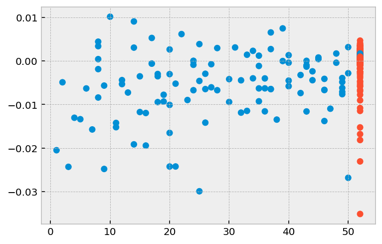
r = cph.compute_residuals(df, 'delta_beta')
r.head()
r = r.join(df[['week', 'arrest']])
r.head()

	fin	race	mar	paro	prio	week	arrest
313	-0.005650	-0.011594	0.012142	-0.027450	-0.020486	1	1
79	-0.005761	-0.005810	0.007687	-0.020926	-0.013373	5	1
60	-0.005783	-0.000147	0.003277	-0.014325	-0.006315	6	1
225	0.014998	-0.041569	0.004855	-0.002254	-0.015725	7	1
138	0.011572	0.005331	-0.004240	0.013036	0.004405	8	1

plt.scatter(r['week'], r['prio'], color=np.where(r['arrest'], '#008fd5', '#fc4f30'))

<matplotlib.collections.PathCollection at 0x11208ab90>

[1] https://stats.stackexchange.com/questions/297740/what-is-the-difference-between-the-different-residuals-in-survival-analysis-cox

[2] http://myweb.uiowa.edu/pbreheny/7210/f15/notes/11-10.pdf