---

自定义回归模型

与单变量模型一样，可以创建自己的自定义参数生存模型。为什么你可能想要这样做？

• 使用已知的概率分布创建新的/扩展AFT模型

• 使用关于主题的领域知识创建一个分段模型

• 迭代并拟合一个更精确的参数模型

lifelines 有一个非常简单的 API 来创建自定义参数回归模型。你只需要定义累积风险函数。例如，恒定风险回归模型的累积风险如下所示：

\[\begin{split}H(t, x) = \frac{t}{\lambda(x)}\\ \lambda(x) = \exp{(\vec{\beta} \cdot \vec{x}^{\,T})}\end{split}\]

其中 \(\beta\) 是我们要优化的未知数。

以下是一些自定义模型的示例。

%matplotlib inline
%config InlineBackend.figure_format = 'retina'

from lifelines.fitters import ParametricRegressionFitter
from autograd import numpy as np
from lifelines.datasets import load_rossi


class ExponentialAFTFitter(ParametricRegressionFitter):

    # this class property is necessary, and should always be a non-empty list of strings.
    _fitted_parameter_names = ['lambda_']

    def _cumulative_hazard(self, params, t, Xs):
        # params is a dictionary that maps unknown parameters to a numpy vector.
        # Xs is a dictionary that maps unknown parameters to a numpy 2d array
        beta = params['lambda_']
        X = Xs['lambda_']
        lambda_ = np.exp(np.dot(X, beta))
        return t / lambda_


rossi = load_rossi()

# the below variables maps {dataframe columns, formulas} to parameters
regressors = {
    # could also be: 'lambda_': rossi.columns.difference(['week', 'arrest'])
    'lambda_': "age + fin + mar + paro + prio + race + wexp + 1"
}

eaf = ExponentialAFTFitter().fit(rossi, 'week', 'arrest', regressors=regressors)
eaf.print_summary()

model	lifelines.ExponentialAFTFitter
duration col	'week'
event col	'arrest'
number of observations	432
number of events observed	114
log-likelihood	-686.37
time fit was run	2020-07-26 22:06:42 UTC

		coef	exp(coef)	se(coef)	coef lower 95%	coef upper 95%	exp(coef) lower 95%	exp(coef) upper 95%	z	p	-log2(p)
param	covariate
lambda_	Intercept	4.05	57.44	0.59	2.90	5.20	18.21	181.15	6.91	<0.005	37.61
	age	0.06	1.06	0.02	0.01	0.10	1.01	1.10	2.55	0.01	6.52
	fin	0.37	1.44	0.19	-0.01	0.74	0.99	2.10	1.92	0.06	4.18
	mar	0.43	1.53	0.38	-0.32	1.17	0.73	3.24	1.12	0.26	1.93
	paro	0.08	1.09	0.20	-0.30	0.47	0.74	1.59	0.42	0.67	0.57
	prio	-0.09	0.92	0.03	-0.14	-0.03	0.87	0.97	-3.03	<0.005	8.65
	race	-0.30	0.74	0.31	-0.91	0.30	0.40	1.35	-0.99	0.32	1.63
	wexp	0.15	1.16	0.21	-0.27	0.56	0.76	1.75	0.69	0.49	1.03

AIC	1388.73
log-likelihood ratio test	31.22 on 7 df
-log2(p) of ll-ratio test	14.11

class DependentCompetingRisksHazard(ParametricRegressionFitter):
    """

    Reference
    --------------
    Frees and Valdez, UNDERSTANDING RELATIONSHIPS USING COPULAS

    """

    _fitted_parameter_names = ["lambda1", "rho1", "lambda2", "rho2", "alpha"]

    def _cumulative_hazard(self, params, T, Xs):
        lambda1 = np.exp(np.dot(Xs["lambda1"], params["lambda1"]))
        lambda2 = np.exp(np.dot(Xs["lambda2"], params["lambda2"]))
        rho2 =    np.exp(np.dot(Xs["rho2"],    params["rho2"]))
        rho1 =    np.exp(np.dot(Xs["rho1"],    params["rho1"]))
        alpha =   np.exp(np.dot(Xs["alpha"],   params["alpha"]))

        return ((T / lambda1) ** rho1 + (T / lambda2) ** rho2) ** alpha


fitter = DependentCompetingRisksHazard(penalizer=0.1)

rossi = load_rossi()
rossi["week"] = rossi["week"] / rossi["week"].max() # scaling often helps with convergence

covariates = {
    "lambda1": rossi.columns.difference(['week', 'arrest']),
    "lambda2": rossi.columns.difference(['week', 'arrest']),
    "rho1": "1",
    "rho2": "1",
    "alpha": "1",
}

fitter.fit(rossi, "week", event_col="arrest", regressors=covariates, timeline=np.linspace(0, 2))
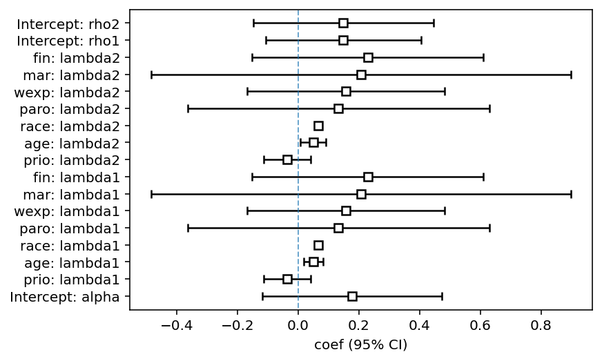
fitter.print_summary(2)

ax = fitter.plot()

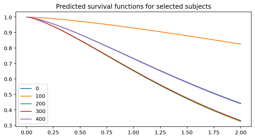
ax = fitter.predict_survival_function(rossi.loc[::100]).plot(figsize=(8, 4))
ax.set_title("Predicted survival functions for selected subjects")

/Users/camerondavidson-pilon/code/lifelines/lifelines/fitters/__init__.py:1985: StatisticalWarning: The diagonal of the variance_matrix_ has negative values. This could be a problem with DependentCompetingRisksHazard's fit to the data.

It's advisable to not trust the variances reported, and to be suspicious of the fitted parameters too.

  warnings.warn(warning_text, exceptions.StatisticalWarning)

model	lifelines.DependentCompetingRisksHazard
duration col	'week'
event col	'arrest'
penalizer	0.1
number of observations	432
number of events observed	114
log-likelihood	-239.19
time fit was run	2020-07-26 22:06:55 UTC

		coef	exp(coef)	se(coef)	coef lower 95%	coef upper 95%	exp(coef) lower 95%	exp(coef) upper 95%	z	p	-log2(p)
param	covariate
lambda1	age	0.05	1.05	0.02	0.02	0.08	1.02	1.09	3.06	<0.005	8.80
	fin	0.23	1.26	0.19	-0.15	0.61	0.86	1.84	1.18	0.24	2.06
	mar	0.21	1.23	0.35	-0.48	0.90	0.62	2.46	0.59	0.56	0.84
	paro	0.13	1.14	0.25	-0.36	0.63	0.69	1.88	0.52	0.60	0.74
	prio	-0.04	0.96	0.04	-0.11	0.04	0.89	1.04	-0.93	0.35	1.50
	race	0.07	1.07	nan	nan	nan	nan	nan	nan	nan	nan
	wexp	0.16	1.17	0.17	-0.17	0.48	0.85	1.62	0.94	0.35	1.53
lambda2	age	0.05	1.05	0.02	0.01	0.09	1.01	1.10	2.34	0.02	5.70
	fin	0.23	1.26	0.19	-0.15	0.61	0.86	1.84	1.18	0.24	2.06
	mar	0.21	1.23	0.35	-0.48	0.90	0.62	2.46	0.59	0.56	0.84
	paro	0.13	1.14	0.25	-0.36	0.63	0.69	1.88	0.52	0.60	0.74
	prio	-0.04	0.96	0.04	-0.11	0.04	0.89	1.04	-0.93	0.35	1.50
	race	0.07	1.07	nan	nan	nan	nan	nan	nan	nan	nan
	wexp	0.16	1.17	0.17	-0.17	0.48	0.85	1.62	0.94	0.35	1.53
rho1	Intercept	0.15	1.16	0.13	-0.11	0.40	0.90	1.50	1.14	0.25	1.98
rho2	Intercept	0.15	1.16	0.15	-0.15	0.44	0.86	1.56	0.99	0.32	1.62
alpha	Intercept	0.18	1.19	0.15	-0.12	0.47	0.89	1.61	1.18	0.24	2.06

AIC	512.38
log-likelihood ratio test	127.04 on 12 df
-log2(p) of ll-ratio test	68.48

Text(0.5, 1.0, 'Predicted survival functions for selected subjects')

治愈模型

假设在我们的总体中有一个子总体永远不会经历感兴趣的事件。或者，对于某些个体来说，事件将在未来非常遥远的时刻发生，几乎等同于无限时间。在这种情况下，个体的生存函数不应渐近地趋近于零，而应趋近于某个正值。描述这种情况的模型有时被称为治愈模型（即个体“治愈”了死亡，因此不再易感）或时间滞后转换模型。

能够使用常见的生存模型并且包含一些“治愈”成分将会很好。假设对于那些会经历感兴趣事件的个体，他们的生存分布是威布尔分布，表示为\(S_W(t)\)。对于随机选择的个体，他们的生存曲线\(S(t)\)是：

\[\begin{split}\begin{align*} S(t) = P(T > t) &= P(\text{cured}) P(T > t\;|\;\text{cured}) + P(\text{not cured}) P(T > t\;|\;\text{not cured}) \\ &= p + (1-p) S_W(t) \end{align*}\end{split}\]

尽管它以一种非常规的形式存在，我们仍然可以确定累积风险（这是生存函数的负对数）：

\[H(t) = -\log{\left(p + (1-p) S_W(t)\right)}\]

from autograd.scipy.special import expit

class CureModel(ParametricRegressionFitter):
    _scipy_fit_method = "SLSQP"
    _scipy_fit_options = {"ftol": 1e-10, "maxiter": 200}

    _fitted_parameter_names = ["lambda_", "beta_", "rho_"]

    def _cumulative_hazard(self, params, T, Xs):
        c = expit(np.dot(Xs["beta_"], params["beta_"]))

        lambda_ = np.exp(np.dot(Xs["lambda_"], params["lambda_"]))
        rho_ = np.exp(np.dot(Xs["rho_"], params["rho_"]))
        sf = np.exp(-(T / lambda_) ** rho_)

        return -np.log((1 - c) + c * sf)


cm = CureModel(penalizer=0.0)

rossi = load_rossi()

covariates = {"lambda_": rossi.columns.difference(['week', 'arrest']), "rho_": "1", "beta_": 'fin + 1'}

cm.fit(rossi, "week", event_col="arrest", regressors=covariates, timeline=np.arange(250))
cm.print_summary(2)

model	lifelines.CureModel
duration col	'week'
event col	'arrest'
number of observations	432
number of events observed	114
log-likelihood	-702.64
time fit was run	2020-07-26 22:07:13 UTC

		coef	exp(coef)	se(coef)	coef lower 95%	coef upper 95%	exp(coef) lower 95%	exp(coef) upper 95%	z	p	-log2(p)
param	covariate
lambda_	age	0.16	1.17	0.05	0.05	0.26	1.06	1.30	2.96	<0.005	8.36
	fin	1.14	3.13	4320.37	-8466.63	8468.92	0.00	inf	0.00	1.00	0.00
	mar	0.35	1.42	0.32	-0.27	0.97	0.76	2.64	1.11	0.27	1.90
	paro	0.26	1.30	0.24	-0.20	0.72	0.82	2.06	1.10	0.27	1.88
	prio	-0.02	0.98	0.04	-0.10	0.06	0.91	1.06	-0.51	0.61	0.71
	race	0.23	1.26	0.28	-0.32	0.79	0.72	2.20	0.82	0.41	1.29
	wexp	0.25	1.28	0.17	-0.08	0.57	0.92	1.78	1.49	0.14	2.86
rho_	Intercept	0.13	1.14	0.08	-0.03	0.29	0.97	1.34	1.57	0.12	3.11
beta_	Intercept	0.18	1.19	0.10	-0.02	0.37	0.98	1.45	1.75	0.08	3.64
	fin	15.80	7.30e+06	0.17	15.46	16.14	5.20e+06	1.03e+07	90.99	<0.005	inf

AIC	1425.29
log-likelihood ratio test	-12.04 on 7 df
-log2(p) of ll-ratio test	-0.00

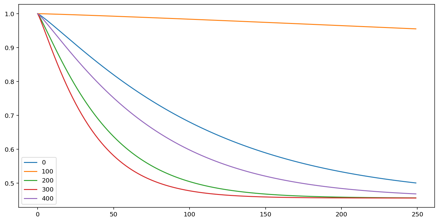
cm.predict_survival_function(rossi.loc[::100]).plot(figsize=(12,6))

<AxesSubplot:>

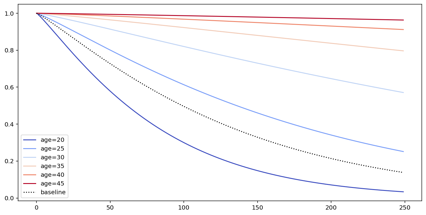
# what's the effect on the survival curve if I vary "age"
fig, ax = plt.subplots(figsize=(12, 6))

cm.plot_covariate_groups(['age'], values=np.arange(20, 50, 5), cmap='coolwarm', ax=ax)

<AxesSubplot:>

样条模型

请查看示例文件夹中的 royston_parmar_splines.py 文件：https://github.com/CamDavidsonPilon/lifelines/tree/master/examples