
[1]:
%matplotlib inline
%config InlineBackend.figure_format = 'retina'

from matplotlib import pyplot as plt
from lifelines import CoxPHFitter
import numpy as np
import pandas as pd
测试比例风险假设
这个Jupyter笔记本是一个关于如何测试和修复比例风险问题的小教程。首先要问的一个重要问题是:我需要关心比例风险假设吗? - 通常答案是否定的。
比例风险假设是所有个体具有相同的风险函数,但前面有一个独特的比例因子。因此,风险函数的形状对所有个体都是相同的,只有每个个体的标量倍数不同。
假设的核心是\(a_i\)不随时间变化,即\(a_i(t) = a_i\)。此外,如果我们将其与另一个对象(称为风险比)的比率进行比较:
对于所有的\(t\)是常数。在本教程中,我们将测试这个非时间变化的假设,并探讨处理违反情况的方法。
[2]:
from lifelines.datasets import load_rossi
rossi = load_rossi()
cph = CoxPHFitter()

cph.fit(rossi, 'week', 'arrest')
[2]:
<lifelines.CoxPHFitter: fitted with 432 total observations, 318 right-censored observations>
[3]:
cph.print_summary(model="untransformed variables", decimals=3)
| model | lifelines.CoxPHFitter |
|---|---|
| duration col | 'week' |
| event col | 'arrest' |
| baseline estimation | breslow |
| number of observations | 432 |
| number of events observed | 114 |
| partial log-likelihood | -658.748 |
| time fit was run | 2020-07-26 22:15:39 UTC |
| model | untransformed variables |
| coef | exp(coef) | se(coef) | coef lower 95% | coef upper 95% | exp(coef) lower 95% | exp(coef) upper 95% | z | p | -log2(p) | |
|---|---|---|---|---|---|---|---|---|---|---|
| covariate | ||||||||||
| fin | -0.379 | 0.684 | 0.191 | -0.755 | -0.004 | 0.470 | 0.996 | -1.983 | 0.047 | 4.398 |
| age | -0.057 | 0.944 | 0.022 | -0.101 | -0.014 | 0.904 | 0.986 | -2.611 | 0.009 | 6.791 |
| race | 0.314 | 1.369 | 0.308 | -0.290 | 0.918 | 0.748 | 2.503 | 1.019 | 0.308 | 1.698 |
| wexp | -0.150 | 0.861 | 0.212 | -0.566 | 0.266 | 0.568 | 1.305 | -0.706 | 0.480 | 1.058 |
| mar | -0.434 | 0.648 | 0.382 | -1.182 | 0.315 | 0.307 | 1.370 | -1.136 | 0.256 | 1.965 |
| paro | -0.085 | 0.919 | 0.196 | -0.469 | 0.299 | 0.626 | 1.348 | -0.434 | 0.665 | 0.589 |
| prio | 0.091 | 1.096 | 0.029 | 0.035 | 0.148 | 1.036 | 1.159 | 3.194 | 0.001 | 9.476 |
| Concordance | 0.640 |
|---|---|
| Partial AIC | 1331.495 |
| log-likelihood ratio test | 33.266 on 7 df |
| -log2(p) of ll-ratio test | 15.370 |
使用check_assumptions检查假设
lifelines 0.16.0 新增了 CoxPHFitter.check_assumptions 方法。该方法将计算统计量以检查比例风险假设,生成图表以检查假设,并提供更多功能。还包括一个选项,可以在控制台显示建议。以下是每个显示信息的详细说明:
首先展示的是用于测试是否存在时变系数的统计测试结果。时变系数意味着协变量相对于基线的影响随时间变化。这意味着违反了比例风险假设。对于每个变量,我们对时间进行了四次转换(这些是常见的时间转换)。如果lifelines拒绝了零假设(即lifelines拒绝了系数不是时变的假设),我们会将此报告给用户。
提供了一些建议,说明如何根据变量的某些汇总统计量来纠正比例风险违规。
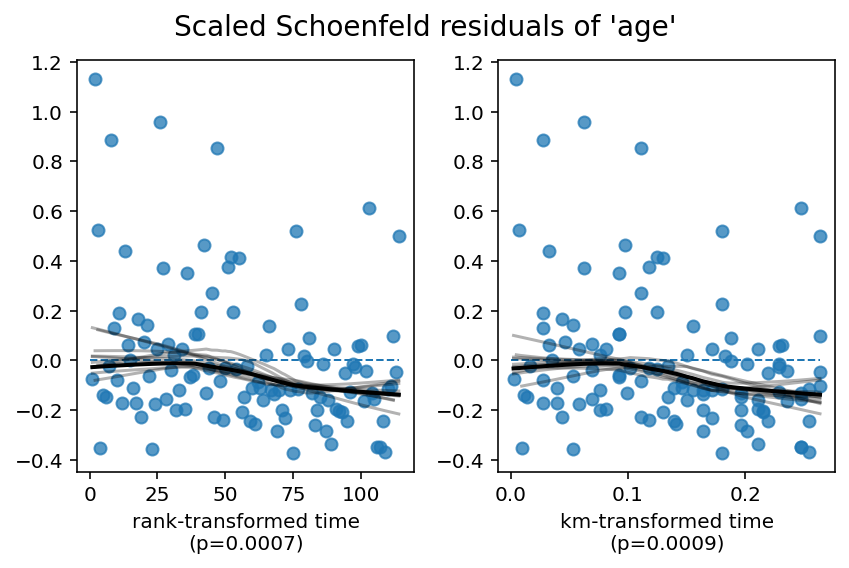
作为对上述统计测试的补充,如果指定了选项
show_plots = True,则会显示所有协变量相对于四种时间变换的缩放Schoenfeld残差的视觉图。还会显示一条拟合的低ess线,以及10条自举低ess线(作为原始低ess线置信区间的近似值)。理想情况下,这条低ess线应该是恒定的(平坦的)。偏离恒定线的情况违反了PH假设。
为什么使用缩放Schoenfeld残差?
这一部分在初次阅读时可以跳过。设\(s_{t,j}\)表示变量\(j\)在时间\(t\)的缩放Schoenfeld残差,\(\hat{\beta_j}\)表示第\(j\)个变量的最大似然估计,\(\beta_j(t)\)表示在(虚构的)允许时变系数的替代模型中的时变系数。Therneau和Grambsch证明了。
比例风险假设意味着 \(\hat{\beta_j} = \beta_j(t)\),因此 \(E[s_{t,j}] = 0\)。这就是上述比例风险检验所检验的内容。从视觉上看,随时间(或时间的某种变换)绘制 \(s_{t,j}\) 是观察 \(E[s_{t,j}] = 0\) 违反情况的好方法,同时结合统计检验。
[4]:
cph.check_assumptions(rossi, p_value_threshold=0.05, show_plots=True)
The ``p_value_threshold`` is set at 0.05. Even under the null hypothesis of no violations, some
covariates will be below the threshold by chance. This is compounded when there are many covariates.
Similarly, when there are lots of observations, even minor deviances from the proportional hazard
assumption will be flagged.

With that in mind, it's best to use a combination of statistical tests and visual tests to determine
the most serious violations. Produce visual plots using ``check_assumptions(..., show_plots=True)``
and looking for non-constant lines. See link [A] below for a full example.
| null_distribution | chi squared |
|---|---|
| degrees_of_freedom | 1 |
| model | <lifelines.CoxPHFitter: fitted with 432 total ... |
| test_name | proportional_hazard_test |
| test_statistic | p | ||
|---|---|---|---|
| age | km | 11.03 | <0.005 |
| rank | 11.45 | <0.005 | |
| fin | km | 0.02 | 0.89 |
| rank | 0.02 | 0.90 | |
| mar | km | 0.60 | 0.44 |
| rank | 0.71 | 0.40 | |
| paro | km | 0.12 | 0.73 |
| rank | 0.13 | 0.71 | |
| prio | km | 0.02 | 0.88 |
| rank | 0.02 | 0.89 | |
| race | km | 1.44 | 0.23 |
| rank | 1.43 | 0.23 | |
| wexp | km | 7.48 | 0.01 |
| rank | 7.31 | 0.01 |
1. Variable 'age' failed the non-proportional test: p-value is 0.0007.
Advice 1: the functional form of the variable 'age' might be incorrect. That is, there may be
non-linear terms missing. The proportional hazard test used is very sensitive to incorrect
functional forms. See documentation in link [D] below on how to specify a functional form.
Advice 2: try binning the variable 'age' using pd.cut, and then specify it in `strata=['age',
...]` in the call in `.fit`. See documentation in link [B] below.
Advice 3: try adding an interaction term with your time variable. See documentation in link [C]
below.
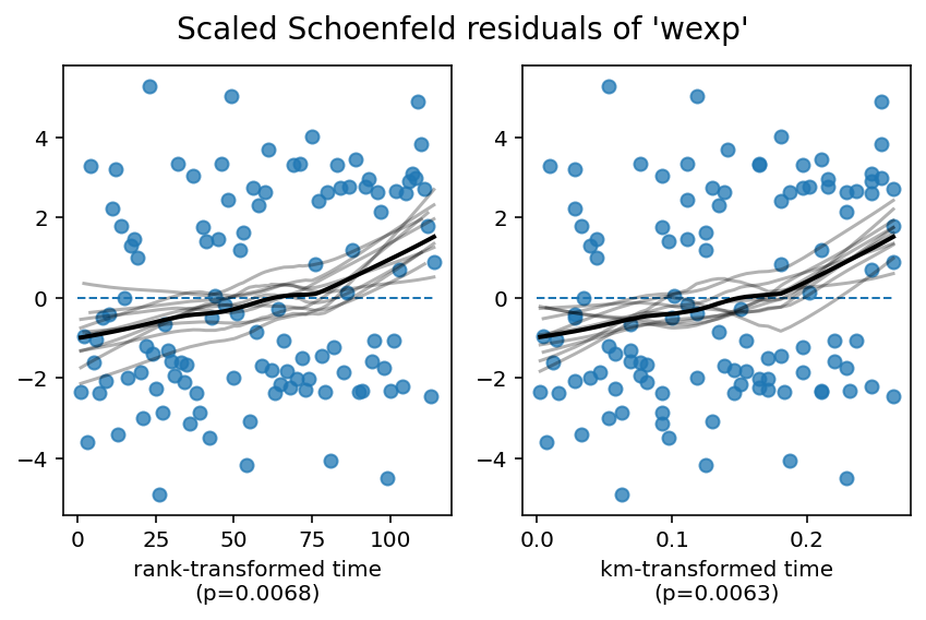
2. Variable 'wexp' failed the non-proportional test: p-value is 0.0063.
Advice: with so few unique values (only 2), you can include `strata=['wexp', ...]` in the call in
`.fit`. See documentation in link [E] below.
---
[A] https://lifelines.readthedocs.io/en/latest/jupyter_notebooks/Proportional%20hazard%20assumption.html
[B] https://lifelines.readthedocs.io/en/latest/jupyter_notebooks/Proportional%20hazard%20assumption.html#Bin-variable-and-stratify-on-it
[C] https://lifelines.readthedocs.io/en/latest/jupyter_notebooks/Proportional%20hazard%20assumption.html#Introduce-time-varying-covariates
[D] https://lifelines.readthedocs.io/en/latest/jupyter_notebooks/Proportional%20hazard%20assumption.html#Modify-the-functional-form
[E] https://lifelines.readthedocs.io/en/latest/jupyter_notebooks/Proportional%20hazard%20assumption.html#Stratification
或者,你可以在check_assumptions之外使用比例风险测试:
[5]:
from lifelines.statistics import proportional_hazard_test

results = proportional_hazard_test(cph, rossi, time_transform='rank')
results.print_summary(decimals=3, model="untransformed variables")
| time_transform | rank |
|---|---|
| null_distribution | chi squared |
| degrees_of_freedom | 1 |
| model | untransformed variables |
| test_name | proportional_hazard_test |
| test_statistic | p | |
|---|---|---|
| age | 11.453 | 0.001 |
| fin | 0.015 | 0.902 |
| mar | 0.709 | 0.400 |
| paro | 0.134 | 0.714 |
| prio | 0.019 | 0.891 |
| race | 1.426 | 0.232 |
| wexp | 7.315 | 0.007 |
分层
在上面的建议中,我们可以看到wexp的基数较小,因此我们可以通过在strata中指定它来轻松解决这个问题。strata是做什么的?让我们回到比例风险假设。
在介绍中,我们说过比例风险假设是
在简单的情况下,可能存在两个具有非常不同基线风险的子组。也就是说,我们可以根据某个变量(我们称之为分层变量)将数据集分成子样本,对所有子样本运行Cox模型,并比较它们的基线风险。如果这些基线风险非常不同,那么显然上述公式是错误的 - \(h(t)\) 是子组基线风险的某种加权平均值。这种不合适的平均基线可能导致 \(a_i\) 具有时间依赖性的影响。更好的模型可能是:
现在我们为每个子组\(G\)有一个独特的基线风险每子组。由于Cox模型的设计方式,系数的推断是相同的(现在有更多的基线风险,并且在子组\(G\)内没有分层变量的变化)。
[6]:
cph.fit(rossi, 'week', 'arrest', strata=['wexp'])
cph.print_summary(model="wexp in strata")
| model | lifelines.CoxPHFitter |
|---|---|
| duration col | 'week' |
| event col | 'arrest' |
| strata | [wexp] |
| baseline estimation | breslow |
| number of observations | 432 |
| number of events observed | 114 |
| partial log-likelihood | -580.89 |
| time fit was run | 2020-07-26 22:15:41 UTC |
| model | wexp in strata |
| coef | exp(coef) | se(coef) | coef lower 95% | coef upper 95% | exp(coef) lower 95% | exp(coef) upper 95% | z | p | -log2(p) | |
|---|---|---|---|---|---|---|---|---|---|---|
| covariate | ||||||||||
| fin | -0.38 | 0.68 | 0.19 | -0.76 | -0.01 | 0.47 | 0.99 | -1.99 | 0.05 | 4.42 |
| age | -0.06 | 0.94 | 0.02 | -0.10 | -0.01 | 0.90 | 0.99 | -2.64 | 0.01 | 6.91 |
| race | 0.31 | 1.36 | 0.31 | -0.30 | 0.91 | 0.74 | 2.49 | 1.00 | 0.32 | 1.65 |
| mar | -0.45 | 0.64 | 0.38 | -1.20 | 0.29 | 0.30 | 1.34 | -1.19 | 0.23 | 2.09 |
| paro | -0.08 | 0.92 | 0.20 | -0.47 | 0.30 | 0.63 | 1.35 | -0.42 | 0.67 | 0.57 |
| prio | 0.09 | 1.09 | 0.03 | 0.03 | 0.15 | 1.04 | 1.16 | 3.16 | <0.005 | 9.33 |
| Concordance | 0.61 |
|---|---|
| Partial AIC | 1173.77 |
| log-likelihood ratio test | 23.77 on 6 df |
| -log2(p) of ll-ratio test | 10.77 |
[7]:
cph.check_assumptions(rossi, show_plots=True)
The ``p_value_threshold`` is set at 0.01. Even under the null hypothesis of no violations, some
covariates will be below the threshold by chance. This is compounded when there are many covariates.
Similarly, when there are lots of observations, even minor deviances from the proportional hazard
assumption will be flagged.

With that in mind, it's best to use a combination of statistical tests and visual tests to determine
the most serious violations. Produce visual plots using ``check_assumptions(..., show_plots=True)``
and looking for non-constant lines. See link [A] below for a full example.
| null_distribution | chi squared |
|---|---|
| degrees_of_freedom | 1 |
| model | <lifelines.CoxPHFitter: fitted with 432 total ... |
| test_name | proportional_hazard_test |
| test_statistic | p | ||
|---|---|---|---|
| age | km | 11.29 | <0.005 |
| rank | 4.62 | 0.03 | |
| fin | km | 0.02 | 0.90 |
| rank | 0.05 | 0.83 | |
| mar | km | 0.53 | 0.47 |
| rank | 1.31 | 0.25 | |
| paro | km | 0.09 | 0.76 |
| rank | 0.00 | 0.97 | |
| prio | km | 0.02 | 0.89 |
| rank | 0.02 | 0.90 | |
| race | km | 1.47 | 0.23 |
| rank | 0.64 | 0.42 |
1. Variable 'age' failed the non-proportional test: p-value is 0.0008.

   Advice 1: the functional form of the variable 'age' might be incorrect. That is, there may be
non-linear terms missing. The proportional hazard test used is very sensitive to incorrect
functional forms. See documentation in link [D] below on how to specify a functional form.

   Advice 2: try binning the variable 'age' using pd.cut, and then specify it in `strata=['age',
...]` in the call in `.fit`. See documentation in link [B] below.

   Advice 3: try adding an interaction term with your time variable. See documentation in link [C]
below.


---
[A]  https://lifelines.readthedocs.io/en/latest/jupyter_notebooks/Proportional%20hazard%20assumption.html
[B]  https://lifelines.readthedocs.io/en/latest/jupyter_notebooks/Proportional%20hazard%20assumption.html#Bin-variable-and-stratify-on-it
[C]  https://lifelines.readthedocs.io/en/latest/jupyter_notebooks/Proportional%20hazard%20assumption.html#Introduce-time-varying-covariates
[D]  https://lifelines.readthedocs.io/en/latest/jupyter_notebooks/Proportional%20hazard%20assumption.html#Modify-the-functional-form
[E]  https://lifelines.readthedocs.io/en/latest/jupyter_notebooks/Proportional%20hazard%20assumption.html#Stratification
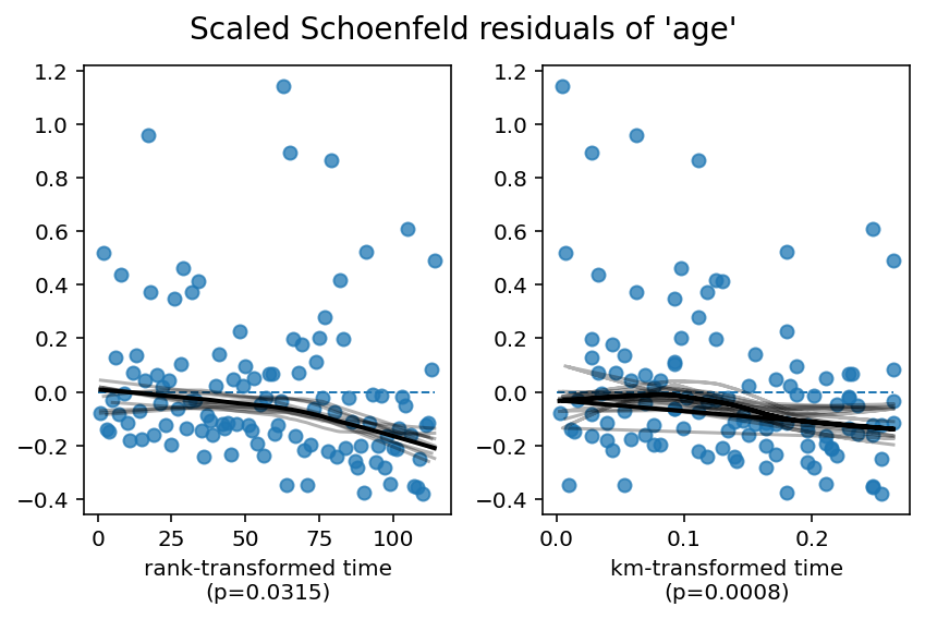
由于age仍然违反了比例风险假设,我们需要更好地建模。从上面的残差图中,我们可以看到年龄的影响随着时间的推移开始变为负值。这在以后会很重要。下面,我们提出了三种处理age的选项。
修改函数形式
比例风险测试在变量的函数形式不正确时非常敏感(即有很多误报)。例如,如果协变量与对数风险之间的关联是非线性的,但模型中只包含线性项,那么比例风险测试可能会产生误报。
建模者可以选择添加二次或三次项,即:
rossi['age**2'] = (rossi['age'] - rossi['age'].mean())**2
rossi['age**3'] = (rossi['age'] - rossi['age'].mean())**3
但我认为包含非线性项的更正确方法是使用基样条:
[9]:
cph.fit(rossi, 'week', 'arrest', strata=['wexp'], formula="bs(age, df=4, lower_bound=10, upper_bound=50) + fin +race + mar + paro + prio")
cph.print_summary(model="spline_model"); print()
cph.check_assumptions(rossi, show_plots=True, p_value_threshold=0.05)
| model | lifelines.CoxPHFitter |
|---|---|
| duration col | 'week' |
| event col | 'arrest' |
| strata | [wexp] |
| baseline estimation | breslow |
| number of observations | 432 |
| number of events observed | 114 |
| partial log-likelihood | -579.36 |
| time fit was run | 2020-07-26 22:19:25 UTC |
| model | spline_model |
| coef | exp(coef) | se(coef) | coef lower 95% | coef upper 95% | exp(coef) lower 95% | exp(coef) upper 95% | z | p | -log2(p) | |
|---|---|---|---|---|---|---|---|---|---|---|
| covariate | ||||||||||
| bs(age, df=4, lower_bound=10, upper_bound=50)[0] | -2.95 | 0.05 | 8.32 | -19.26 | 13.37 | 0.00 | 6.39e+05 | -0.35 | 0.72 | 0.47 |
| bs(age, df=4, lower_bound=10, upper_bound=50)[1] | -5.48 | 0.00 | 6.23 | -17.69 | 6.73 | 0.00 | 839.48 | -0.88 | 0.38 | 1.40 |
| bs(age, df=4, lower_bound=10, upper_bound=50)[2] | -3.69 | 0.03 | 8.88 | -21.10 | 13.72 | 0.00 | 9.09e+05 | -0.42 | 0.68 | 0.56 |
| bs(age, df=4, lower_bound=10, upper_bound=50)[3] | -6.02 | 0.00 | 6.75 | -19.26 | 7.21 | 0.00 | 1351.35 | -0.89 | 0.37 | 1.43 |
| fin | -0.37 | 0.69 | 0.19 | -0.75 | 0.01 | 0.47 | 1.01 | -1.93 | 0.05 | 4.22 |
| race | 0.35 | 1.42 | 0.31 | -0.26 | 0.95 | 0.77 | 2.60 | 1.13 | 0.26 | 1.95 |
| mar | -0.39 | 0.67 | 0.38 | -1.15 | 0.36 | 0.32 | 1.43 | -1.02 | 0.31 | 1.71 |
| paro | -0.10 | 0.90 | 0.20 | -0.49 | 0.28 | 0.61 | 1.33 | -0.53 | 0.60 | 0.75 |
| prio | 0.09 | 1.10 | 0.03 | 0.04 | 0.15 | 1.04 | 1.16 | 3.22 | <0.005 | 9.59 |
| Concordance | 0.62 |
|---|---|
| Partial AIC | 1176.72 |
| log-likelihood ratio test | 26.82 on 9 df |
| -log2(p) of ll-ratio test | 9.38 |
Proportional hazard assumption looks okay.
我们可能仍然存在一些潜在的违规,但已经少了很多。此外,有趣的是,当我们为age包含这些非线性项时,wexp的比例违规消失了。通常,改变一个变量的函数形式会影响其他变量的比例测试,通常是积极的。因此,如果我们愿意,可以移除strata=['wexp']。
分箱变量并对其进行分层
提出的第二个选项是将变量分箱为等大小的箱,并像我们对wexp所做的那样进行分层。这里在估计和信息损失之间存在权衡。如果我们有较大的箱,我们将丢失信息(因为不同的值现在被分箱在一起),但我们需要估计较少的新基线风险。另一方面,使用较小的箱,我们允许age数据具有最大的“摆动空间”,但必须计算许多基线风险,每个基线风险的样本量较小。像大多数事情一样,最佳值介于两者之间。
[10]:
rossi_strata_age = rossi.copy()
rossi_strata_age['age_strata'] = pd.cut(rossi_strata_age['age'], np.arange(0, 80, 3))

rossi_strata_age[['age', 'age_strata']].head()
[10]:
| age | age_strata | |
|---|---|---|
| 0 | 27 | (24, 27] |
| 1 | 18 | (15, 18] |
| 2 | 19 | (18, 21] |
| 3 | 23 | (21, 24] |
| 4 | 19 | (18, 21] |
[11]:
# drop the original, redundant, age column
rossi_strata_age = rossi_strata_age.drop('age', axis=1)
cph.fit(rossi_strata_age, 'week', 'arrest', strata=['age_strata', 'wexp'])
[11]:
<lifelines.CoxPHFitter: fitted with 432 total observations, 318 right-censored observations>
[12]:
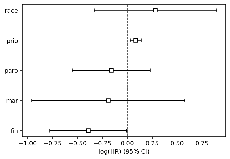
cph.print_summary(3, model="stratified age and wexp")
cph.plot()
| model | lifelines.CoxPHFitter |
|---|---|
| duration col | 'week' |
| event col | 'arrest' |
| strata | [age_strata, wexp] |
| baseline estimation | breslow |
| number of observations | 432 |
| number of events observed | 114 |
| partial log-likelihood | -392.443 |
| time fit was run | 2020-07-26 22:19:46 UTC |
| model | stratified age and wexp |
| coef | exp(coef) | se(coef) | coef lower 95% | coef upper 95% | exp(coef) lower 95% | exp(coef) upper 95% | z | p | -log2(p) | |
|---|---|---|---|---|---|---|---|---|---|---|
| covariate | ||||||||||
| fin | -0.395 | 0.674 | 0.197 | -0.781 | -0.009 | 0.458 | 0.991 | -2.004 | 0.045 | 4.472 |
| race | 0.280 | 1.324 | 0.313 | -0.334 | 0.895 | 0.716 | 2.447 | 0.895 | 0.371 | 1.431 |
| mar | -0.194 | 0.824 | 0.392 | -0.961 | 0.574 | 0.382 | 1.776 | -0.494 | 0.621 | 0.687 |
| paro | -0.163 | 0.849 | 0.200 | -0.555 | 0.228 | 0.574 | 1.256 | -0.818 | 0.413 | 1.275 |
| prio | 0.080 | 1.084 | 0.028 | 0.025 | 0.135 | 1.025 | 1.145 | 2.854 | 0.004 | 7.857 |
| Concordance | 0.582 |
|---|---|
| Partial AIC | 794.887 |
| log-likelihood ratio test | 13.247 on 5 df |
| -log2(p) of ll-ratio test | 5.562 |
[12]:
<AxesSubplot:xlabel='log(HR) (95% CI)'>
[13]:
cph.check_assumptions(rossi_strata_age)
Proportional hazard assumption looks okay.
引入时变协变量
我们纠正违反比例风险假设的变量的第二个选择是直接建模时变成分。这分为两个步骤。首先是将你的数据集转换为事件格式。这意味着我们将一个主题从单行拆分为\(n\)新行,每个新行代表该主题的某个时间段。变量在这些新时间段内是静态的也没关系——我们稍后会引入一些时变协变量。
请参阅以下如何在lifelines中执行此操作:
[14]:
from lifelines.utils import to_episodic_format

# the time_gaps parameter specifies how large or small you want the periods to be.
rossi_long = to_episodic_format(rossi, duration_col='week', event_col='arrest', time_gaps=1.)
rossi_long.head(25)
[14]:
| stop | start | arrest | age | fin | id | mar | paro | prio | race | wexp | |
|---|---|---|---|---|---|---|---|---|---|---|---|
| 0 | 1.0 | 0.0 | 0 | 27 | 0 | 0 | 0 | 1 | 3 | 1 | 0 |
| 1 | 2.0 | 1.0 | 0 | 27 | 0 | 0 | 0 | 1 | 3 | 1 | 0 |
| 2 | 3.0 | 2.0 | 0 | 27 | 0 | 0 | 0 | 1 | 3 | 1 | 0 |
| 3 | 4.0 | 3.0 | 0 | 27 | 0 | 0 | 0 | 1 | 3 | 1 | 0 |
| 4 | 5.0 | 4.0 | 0 | 27 | 0 | 0 | 0 | 1 | 3 | 1 | 0 |
| 5 | 6.0 | 5.0 | 0 | 27 | 0 | 0 | 0 | 1 | 3 | 1 | 0 |
| 6 | 7.0 | 6.0 | 0 | 27 | 0 | 0 | 0 | 1 | 3 | 1 | 0 |
| 7 | 8.0 | 7.0 | 0 | 27 | 0 | 0 | 0 | 1 | 3 | 1 | 0 |
| 8 | 9.0 | 8.0 | 0 | 27 | 0 | 0 | 0 | 1 | 3 | 1 | 0 |
| 9 | 10.0 | 9.0 | 0 | 27 | 0 | 0 | 0 | 1 | 3 | 1 | 0 |
| 10 | 11.0 | 10.0 | 0 | 27 | 0 | 0 | 0 | 1 | 3 | 1 | 0 |
| 11 | 12.0 | 11.0 | 0 | 27 | 0 | 0 | 0 | 1 | 3 | 1 | 0 |
| 12 | 13.0 | 12.0 | 0 | 27 | 0 | 0 | 0 | 1 | 3 | 1 | 0 |
| 13 | 14.0 | 13.0 | 0 | 27 | 0 | 0 | 0 | 1 | 3 | 1 | 0 |
| 14 | 15.0 | 14.0 | 0 | 27 | 0 | 0 | 0 | 1 | 3 | 1 | 0 |
| 15 | 16.0 | 15.0 | 0 | 27 | 0 | 0 | 0 | 1 | 3 | 1 | 0 |
| 16 | 17.0 | 16.0 | 0 | 27 | 0 | 0 | 0 | 1 | 3 | 1 | 0 |
| 17 | 18.0 | 17.0 | 0 | 27 | 0 | 0 | 0 | 1 | 3 | 1 | 0 |
| 18 | 19.0 | 18.0 | 0 | 27 | 0 | 0 | 0 | 1 | 3 | 1 | 0 |
| 19 | 20.0 | 19.0 | 1 | 27 | 0 | 0 | 0 | 1 | 3 | 1 | 0 |
| 20 | 1.0 | 0.0 | 0 | 18 | 0 | 1 | 0 | 1 | 8 | 1 | 0 |
| 21 | 2.0 | 1.0 | 0 | 18 | 0 | 1 | 0 | 1 | 8 | 1 | 0 |
| 22 | 3.0 | 2.0 | 0 | 18 | 0 | 1 | 0 | 1 | 8 | 1 | 0 |
| 23 | 4.0 | 3.0 | 0 | 18 | 0 | 1 | 0 | 1 | 8 | 1 | 0 |
| 24 | 5.0 | 4.0 | 0 | 18 | 0 | 1 | 0 | 1 | 8 | 1 | 0 |
每个主题都被赋予一个新的id(但如果数据框中已经提供了,也可以指定)。这个id用于随时间跟踪主题。请注意,arrest列在他们(可能的)事件之前的所有时期也为0。
上面我提到了修正age有两个步骤。第一步是转换为事件格式。第二步是在age和stop之间创建一个交互项。这是一个随时间变化的变量。
由于我们正在处理一个片段数据集,我们必须使用CoxTimeVaryingFitter而不是CoxPHFitter。
[15]:
rossi_long['time*age'] = rossi_long['age'] * rossi_long['stop']
[16]:
from lifelines import CoxTimeVaryingFitter
ctv = CoxTimeVaryingFitter()

ctv.fit(rossi_long,
        id_col='id',
        event_col='arrest',
        start_col='start',
        stop_col='stop',
        strata=['wexp'])
[16]:
<lifelines.CoxTimeVaryingFitter: fitted with 19809 periods, 432 subjects, 114 events>
[17]:
ctv.print_summary(3, model="age * time interaction")
| model | lifelines.CoxTimeVaryingFitter |
|---|---|
| event col | 'arrest' |
| strata | [wexp] |
| number of subjects | 432 |
| number of periods | 19809 |
| number of events | 114 |
| partial log-likelihood | -575.080 |
| time fit was run | 2020-07-26 22:19:49 UTC |
| model | age * time interaction |
| coef | exp(coef) | se(coef) | coef lower 95% | coef upper 95% | exp(coef) lower 95% | exp(coef) upper 95% | z | p | -log2(p) | |
|---|---|---|---|---|---|---|---|---|---|---|
| covariate | ||||||||||
| age | 0.073 | 1.075 | 0.040 | -0.005 | 0.151 | 0.995 | 1.163 | 1.830 | 0.067 | 3.893 |
| fin | -0.386 | 0.680 | 0.191 | -0.760 | -0.011 | 0.468 | 0.989 | -2.018 | 0.044 | 4.520 |
| mar | -0.397 | 0.672 | 0.382 | -1.147 | 0.352 | 0.318 | 1.422 | -1.039 | 0.299 | 1.743 |
| paro | -0.098 | 0.907 | 0.196 | -0.481 | 0.285 | 0.618 | 1.330 | -0.501 | 0.616 | 0.698 |
| prio | 0.090 | 1.094 | 0.029 | 0.034 | 0.146 | 1.035 | 1.158 | 3.152 | 0.002 | 9.267 |
| race | 0.295 | 1.343 | 0.308 | -0.310 | 0.899 | 0.733 | 2.458 | 0.955 | 0.340 | 1.558 |
| time*age | -0.005 | 0.995 | 0.002 | -0.008 | -0.002 | 0.992 | 0.998 | -3.337 | 0.001 | 10.203 |
| Partial AIC | 1164.160 |
|---|---|
| log-likelihood ratio test | 35.386 on 7 df |
| -log2(p) of ll-ratio test | 16.689 |
[ ]:
ctv.plot()
<AxesSubplot:xlabel='log(HR) (95% CI)'>
在上述的age缩放Schoenfeld残差图中,我们可以看到对于较高的时间值存在轻微的负面影响。这在CoxTimeVaryingFitter的输出中得到了确认:我们看到time*age的系数是-0.005。
结论
使用任一选项的点估计和标准误差都非常接近,我们可以有信心地认为任一方法都可以继续进行。
我需要关心比例风险假设吗?
你可能会惊讶地发现,通常你不需要关心比例风险假设。有很多原因可以解释这一点:
如果你的目标是生存预测,那么你不需要关心比例风险。你的目标是最大化某个分数,与预测如何生成无关。
给定足够大的样本量,即使比例风险的非常小的违反也会显现出来。
有合理的理由假设所有数据集都会违反比例风险假设。这在Stensrud & Hernán的“为什么要测试比例风险?”[1]中有详细说明。
“即使风险不成比例,改变模型以适应一组假设从根本上改变了科学问题。正如Tukey所说,‘宁愿对确切问题的近似答案,也不愿对近似问题的确切答案。’如果你在存在非比例风险的情况下拟合Cox模型,净效应是什么?稍微降低了一些效力。事实上,你可以通过稳健的标准误差(指定robust=True)恢复大部分效力。在这种情况下,(指数化的)模型系数的解释是风险比的时间加权平均值——我每次都会这样做。”来自AdamO,稍作修改以适应lifelines [2]
鉴于上述考虑,现状仍然是检查比例风险。因此,如果您避免测试比例风险,请确保理解并能够回答为什么您避免测试。
Stensrud MJ, Hernán MA. 为什么要测试比例风险? JAMA. 在线发布于2020年3月13日. doi:10.1001/jama.2020.1267
AdamO (https://stats.stackexchange.com/users/8013/adamo), 检查比例风险假设, URL (版本: 2019-04-05): https://stats.stackexchange.com/q/400981
[ ]: