两次相关函数
使用QuTiP的时间演化函数(例如mesolve和mcsolve),可以将状态向量或密度矩阵从初始状态\(t_0\)演化到任意时间\(t\),\(\rho(t)=V(t, t_0)\left\{\rho(t_0)\right\}\),其中\(V(t, t_0)\)是由运动方程定义的传播子。然后可以使用生成的密度矩阵来评估任意组合的同时算符的期望值。
为了计算形式为 \(\left
因此,我们首先使用QuTiP演化求解器之一,以\(\rho(0)\)作为初始状态计算\(\rho(t)=V(t, 0)\left\{\rho(0)\right\}\),然后再次使用相同的求解器,以\(B\rho(t)\)作为初始状态计算\(V(t+\tau, t)\left\{B\rho(t)\right\}\)。
请注意,如果初始状态是稳态,那么 \(\rho(t)=V(t, 0)\left\{\rho_{\rm ss}\right\}=\rho_{\rm ss}\) 并且
这是独立于\(t\)的,因此我们只有一个时间坐标\(\tau\)。
QuTiP 提供了一系列函数,用于帮助计算双时间相关函数的过程。可用的函数及其用法如下表所示。这些函数中的每一个都可以使用以下演化求解器之一:主方程、指数级数和蒙特卡洛。求解器的选择由可选参数 solver 定义。
QuTiP 函数 |
相关函数 |
|---|---|
|
\(\left |
|
\(\left |
|
\(\left |
|
\(\left |
|
\(\left |
最常见的用例是计算两个时间相关函数 \(\leftcorrelation_2op_1t 使用合理的默认值执行此任务,但仅允许使用 mesolve 求解器。从 QuTiP 5.0 开始,我们添加了 correlation_3op。此函数还可以计算具有两个或三个运算符以及一个或两个时间的相关函数。最重要的是,此函数接受替代求解器,例如 brmesolve。
稳态相关函数
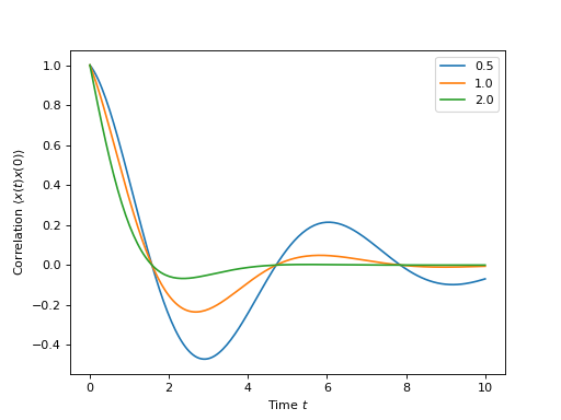
以下代码演示了如何计算具有三种不同弛豫率的泄漏腔的\(\left
times = np.linspace(0,10.0,200)
a = destroy(10)
x = a.dag() + a
H = a.dag() * a

corr1 = correlation_2op_1t(H, None, times, [np.sqrt(0.5) * a], x, x)
corr2 = correlation_2op_1t(H, None, times, [np.sqrt(1.0) * a], x, x)
corr3 = correlation_2op_1t(H, None, times, [np.sqrt(2.0) * a], x, x)

plt.figure()
plt.plot(times, np.real(corr1))
plt.plot(times, np.real(corr2))
plt.plot(times, np.real(corr3))
plt.legend(['0.5','1.0','2.0'])
plt.xlabel(r'Time $t$')
plt.ylabel(r'Correlation $\left<x(t)x(0)\right>$')
plt.show()
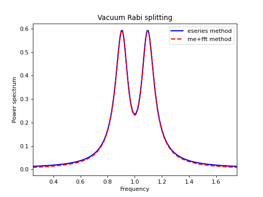
发射光谱
给定一个相关函数 \(\left
在QuTiP中,我们可以使用spectrum来计算\(S(\omega)\),该函数首先使用其中一个时间相关的求解器计算相关函数,然后半解析地执行傅里叶变换,或者我们可以使用函数spectrum_correlation_fft来使用FFT数值计算给定相关数据的傅里叶变换。
以下示例演示了如何使用这两个函数来获取发射功率谱。
import numpy as np
from matplotlib import pyplot
import qutip

N = 4                      # number of cavity fock states
wc = wa = 1.0 * 2 * np.pi  # cavity and atom frequency
g  = 0.1 * 2 * np.pi       # coupling strength
kappa = 0.75               # cavity dissipation rate
gamma = 0.25               # atom dissipation rate

# Jaynes-Cummings Hamiltonian
a  = qutip.tensor(qutip.destroy(N), qutip.qeye(2))
sm = qutip.tensor(qutip.qeye(N), qutip.destroy(2))
H = wc*a.dag()*a + wa*sm.dag()*sm + g*(a.dag()*sm + a*sm.dag())

# collapse operators
n_th = 0.25
c_ops = [
    np.sqrt(kappa * (1 + n_th)) * a,
    np.sqrt(kappa * n_th) * a.dag(),
    np.sqrt(gamma) * sm,
]

# calculate the correlation function using the mesolve solver, and then fft to
# obtain the spectrum. Here we need to make sure to evaluate the correlation
# function for a sufficient long time and sufficiently high sampling rate so
# that the discrete Fourier transform (FFT) captures all the features in the
# resulting spectrum.
tlist = np.linspace(0, 100, 5000)
corr = qutip.correlation_2op_1t(H, None, tlist, c_ops, a.dag(), a)
wlist1, spec1 = qutip.spectrum_correlation_fft(tlist, corr)


# calculate the power spectrum using spectrum, which internally uses essolve
# to solve for the dynamics (by default)
wlist2 = np.linspace(0.25, 1.75, 200) * 2 * np.pi
spec2 = qutip.spectrum(H, wlist2, c_ops, a.dag(), a)

# plot the spectra
fig, ax = pyplot.subplots(1, 1)
ax.plot(wlist1 / (2 * np.pi), spec1, 'b', lw=2, label='eseries method')
ax.plot(wlist2 / (2 * np.pi), spec2, 'r--', lw=2, label='me+fft method')
ax.legend()
ax.set_xlabel('Frequency')
ax.set_ylabel('Power spectrum')
ax.set_title('Vacuum Rabi splitting')
ax.set_xlim(wlist2[0]/(2*np.pi), wlist2[-1]/(2*np.pi))
plt.show()
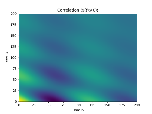
非稳态相关函数
更一般地,我们也可以计算类似\(\leftcorrelation_2op_2t来评估此类相关函数。此函数的默认行为是返回一个矩阵,其中包含作为两个时间坐标(\(t_1\)和\(t_2\))的函数的相关性。
import numpy as np
import matplotlib.pyplot as plt
import qutip

times = np.linspace(0, 10.0, 200)
a = qutip.destroy(10)
x = a.dag() + a
H = a.dag() * a
alpha = 2.5
rho0 = qutip.coherent_dm(10, alpha)
corr = qutip.correlation_2op_2t(H, rho0, times, times, [np.sqrt(0.25) * a], x, x)

plt.pcolor(np.real(corr))
plt.xlabel(r'Time $t_2$')
plt.ylabel(r'Time $t_1$')
plt.title(r'Correlation $\left<x(t)x(0)\right>$')
plt.show()
然而,在某些情况下,我们可能对形式为\(\leftcorrelation_2op_2t函数。correlation_2op_2t函数随后返回一个向量,其中包含与taulist(第四个参数)中的时间对应的相关值。
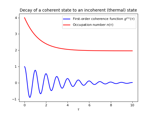
示例:一阶光学相干函数
这个例子演示了如何计算非稳态初始状态下的相关函数形式 \(\left
import numpy as np
import matplotlib.pyplot as plt
import qutip

N = 15
taus = np.linspace(0,10.0,200)
a = qutip.destroy(N)
H = 2 * np.pi * a.dag() * a

# collapse operator
G1 = 0.75
n_th = 2.00  # bath temperature in terms of excitation number
c_ops = [np.sqrt(G1 * (1 + n_th)) * a, np.sqrt(G1 * n_th) * a.dag()]

# start with a coherent state
rho0 = qutip.coherent_dm(N, 2.0)

# first calculate the occupation number as a function of time
n = qutip.mesolve(H, rho0, taus, c_ops, e_ops=[a.dag() * a]).expect[0]

# calculate the correlation function G1 and normalize with n to obtain g1
G1 = qutip.correlation_2op_1t(H, rho0, taus, c_ops, a.dag(), a)
g1 = np.array(G1) / np.sqrt(n[0] * np.array(n))

plt.plot(taus, np.real(g1), 'b', lw=2)
plt.plot(taus, n, 'r', lw=2)
plt.title('Decay of a coherent state to an incoherent (thermal) state')
plt.xlabel(r'$\tau$')
plt.legend([
    r'First-order coherence function $g^{(1)}(\tau)$',
    r'Occupation number $n(\tau)$',
])
plt.show()
为了方便起见,计算一阶相干函数的步骤已收集在函数 coherence_function_g1 中。
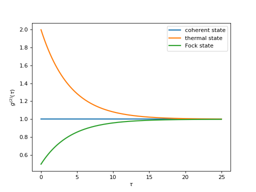
示例:二阶光学相干函数
二阶光学相干函数,具有时间延迟 \(\tau\),定义为
对于一个相干态\(g^{(2)}(\tau) = 1\),对于一个热态\(g^{(2)}(\tau=0) = 2\),并且它随时间减少(光子聚集,它们倾向于一起出现),而对于一个具有\(n\)个光子的福克态\(g^{(2)}(\tau = 0) = n(n - 1)/n^2 < 1\),并且它随时间增加(反聚集光子,更可能在时间上分开到达)。
要使用QuTiP计算这种类型的相关函数,我们可以使用correlation_3op_1t,它计算形式为\(\left
以下代码计算并绘制了相干态、热态和福克态的\(g^{(2)}(\tau)\)作为\(\tau\)的函数。
import numpy as np
import matplotlib.pyplot as plt
import qutip

N = 25
taus = np.linspace(0, 25.0, 200)
a = qutip.destroy(N)
H = 2 * np.pi * a.dag() * a

kappa = 0.25
n_th = 2.0  # bath temperature in terms of excitation number
c_ops = [np.sqrt(kappa * (1 + n_th)) * a, np.sqrt(kappa * n_th) * a.dag()]

states = [
    {'state': qutip.coherent_dm(N, np.sqrt(2)), 'label': "coherent state"},
    {'state': qutip.thermal_dm(N, 2), 'label': "thermal state"},
    {'state': qutip.fock_dm(N, 2), 'label': "Fock state"},
]

fig, ax = plt.subplots(1, 1)

for state in states:
    rho0 = state['state']

    # first calculate the occupation number as a function of time
    n = qutip.mesolve(H, rho0, taus, c_ops, e_ops=[a.dag() * a]).expect[0]

    # calculate the correlation function G2 and normalize with n(0)n(t) to
    # obtain g2
    G2 = qutip.correlation_3op_1t(H, rho0, taus, c_ops, a.dag(), a.dag()*a, a)
    g2 = np.array(G2) / (n[0] * np.array(n))

    ax.plot(taus, np.real(g2), label=state['label'], lw=2)

ax.legend(loc=0)
ax.set_xlabel(r'$\tau$')
ax.set_ylabel(r'$g^{(2)}(\tau)$')
plt.show()
为了方便起见,计算二阶相干函数的步骤已收集在函数 coherence_function_g2 中。