流数据时间序列的增量矩阵剖面#
![]()
现在您对如何计算矩阵剖面有了基本的了解,在这个简短的教程中,我们将演示如何在您拥有流(在线)数据时,增量更新您的矩阵剖面,使用 stumpy.stumpi (“STUMP 增量”) 函数。您可以通过阅读 矩阵剖面 I 论文的 G 节和本论文的第 4.6 节及表 5 来了解更多关于这种方法的细节。
开始使用#
让我们导入创建和分析随机生成的时间序列数据集所需的包。
import numpy as np
import stumpy
import numpy.testing as npt
import time
生成一些随机时间序列数据#
想象一下我们有一个物联网传感器,在过去的14天里每小时收集一次数据。这意味着到目前为止,我们已经积累了14 * 24 = 336个数据点,我们的数据集可能看起来是这样的:
T = np.random.rand(336)
而且,也许我们从经验中知道,一个有趣的主题或异常可能在12小时(滑动)时间窗口内被检测到:
m = 12
典型的批量分析#
使用 stumpy.stump 通过批处理计算矩阵轮廓非常简单:
mp = stumpy.stump(T, m)
但是随着T的长度随着每小时的流逝而增加,计算矩阵轮廓将需要越来越多的时间,因为stumpy.stump实际上会重新计算时间序列中所有子序列之间的所有成对距离。这非常耗时!相反,对于流数据,我们希望找到一种方法,将新来的(单个)数据点与其所处的子序列进行比较,并与其余时间序列进行比较(即,计算距离轮廓)并更新现有的矩阵轮廓。幸运的是,这可以通过stumpy.stumpi或“STUMP增量”轻松完成。
使用 STUMPI 进行流式(在线)分析#
在我们等待下一个数据点 t 到来时,我们可以利用现有的数据初始化我们的流对象:
stream = stumpy.stumpi(T, m, egress=False) # Don't egress/remove the oldest data point when streaming
当新的数据点 t 到达时:
t = np.random.rand()
我们可以将 t 附加到我们的 stream,并轻松地在后台更新矩阵配置文件 P 和矩阵配置文件索引 I:
stream.update(t)
在后台, t 已被追加到现有时间序列中,它会自动将新的子序列与所有现有的子序列进行比较并更新历史值。它还会确定哪个现有子序列是新的子序列的最近邻,并将此信息附加到矩阵剖面中。这可以继续进行,例如,再进行 1,000 次迭代(或无限期)随着额外数据的流入:
for i in range(1000):
t = np.random.rand()
stream.update(t)
重要的是要重申,增量 stumpy.stumpi 与批处理 stumpy.stump 的不同之处在于,它不会浪费时间重新计算任何过去的成对距离。 stumpy.stumpi 只花时间计算新的距离,然后在必要时更新相应的数组,因此,它真的很快!
验证#
矩阵剖面#
现在,这种关于流式(在线)数据的“快速更新”声明可能会让人感到奇怪或似乎是魔法,因此,首先,让我们验证增量 stumpy.stumpi 的输出与执行批处理 stumpy.stump 是相同的。我们从包含 64 个数据点的完整时间序列开始,计算完整的矩阵模型:
T_full = np.random.rand(64)
m = 8
mp = stumpy.stump(T_full, m)
P_full = mp[:, 0]
I_full = mp[:, 1]
在STUMPY版本1.12.0之后添加
可以通过 P_ 属性直接访问矩阵谱距离,通过 I_ 属性访问矩阵谱索引:
mp = stumpy.stump(T, m)
print(mp.P_, mp.I_) # print the matrix profile and the matrix profile indices
此外,左侧和右侧矩阵轮廓索引还可以通过 left_I_ 和 right_I_ 属性分别访问。
接下来,对于 stumpy.stumpi,我们将只从完整的时间序列中开始使用前 10 个元素,然后逐个增量地流入额外的数据点:
# Start with half of the full length time series and initialize inputs
T_stream = T_full[:10].copy()
stream = stumpy.stumpi(T_stream, m, egress=False) # Don't remove/egress the oldest data point when streaming
# Incrementally add one new data point at a time and update the matrix profile
for i in range(len(T_stream), len(T_full)):
t = T_full[i]
stream.update(t)
现在我们完成了,让我们检查并验证:
stream.T == T_fullstream.P == P_fullstream.I == I_full
npt.assert_almost_equal(stream.T_, T_full)
npt.assert_almost_equal(stream.P_, P_full)
npt.assert_almost_equal(stream.I_, I_full)
没有错误!这意味着 stump.stumpi 确实产生了我们所期望的正确矩阵轮廓结果。
性能#
我们基本上声称,使用 stumpy.stumpi 逐步更新我们的矩阵概况在总计算时间上比使用 stumpy.stump 进行完全配对距离计算要快得多,因为每当新数据点到达时。让我们通过取一个长度为 1,000 数据点的完整时间序列来实际比较时间,我们用时间序列的前 2%(即前 20 个点)初始化这两种方法,并在每次迭代之前附加一个新的数据点,然后重新计算矩阵概况:
T_full = np.random.rand(1_000)
T_stream = T_full[:20].copy()
m = 10
# `stumpy.stump` timing
start = time.time()
mp = stumpy.stump(T_stream, m)
for i in range(20, len(T_full)):
T_stream = np.append(T_stream, T_full[i])
mp = stumpy.stump(T_stream, m)
stump_time = time.time() - start
# `stumpy.stumpi` timing
stream = stumpy.stumpi(T_stream, m, egress=False) # Don't egress/remove the oldest data point when streaming
start = time.time()
for i in range(20, len(T_full)):
t = T_full[i]
stream.update(t)
stumpi_time = time.time() - start
print(f"stumpy.stump: {np.round(stump_time,1)}s")
print(f"stumpy.stumpi: {np.round(stumpi_time, 1)}s")
stumpy.stump: 2.7s
stumpy.stumpi: 0.3s
撇开更多CPU会加速这两种方法这一事实,我们清楚地看到增量 stumpy.stumpi 在处理流数据时比批处理 stumpy.stump 快一个到两个数量级。事实上,对于当前的硬件,平均而言,stumpy.stump 分析每个新矩阵轮廓大约需要 0.1 秒。因此,如果每秒出现超过 10 个新数据点,那么你将无法跟上。相比之下,stumpy.stumpi 应该能够舒适地处理和处理 ~450+ 个每秒的新数据点,使用相当适中的硬件。此外,批处理 stumpy.stump 的计算复杂度为 O(n^2),随着越来越多的数据点被添加到现有时间序列中,它会变得更慢,而 stumpy.stumpi 本质上为 O(1),将继续保持高性能。
事实上,如果你 不 在意维护最旧的数据点及其与最新数据点的关系(即,你只关心维持一个固定大小的滑动窗口),那么你可以通过告诉 stumpy.stumpi 移除/淘汰最旧的数据点(以及其对应的矩阵剖面信息)来稍微提高性能,当我们实例化我们的流对象时,通过设置参数 egress=True (请注意,这实际上是默认行为):
stream = stumpy.stumpi(T_stream, m, egress=True) # Egressing/removing the oldest data point is the default behavior!
现在,当我们处理上面的相同数据时:
# `stumpy.stumpi` timing with egress
stream = stumpy.stumpi(T_stream, m, egress=True)
start = time.time()
for i in range(200, len(T_full)):
t = T_full[i]
stream.update(t)
stumpi_time = time.time() - start
print(f"stumpy.stumpi: {np.round(stumpi_time, 1)}s")
stumpy.stumpi: 0.2s
一个视觉示例#
现在我们理解了如何使用流数据计算和更新我们的矩阵剖面,让我们用一个真实的数据集来探索这个问题,其中有一个已知的模式,并看看 stumpy.stumpi 是否能够正确识别何时遇到全局模式(花样)。
检索和加载数据#
首先让我们导入一些额外的Python包,然后检索我们的标准“Steamgen数据集”:
%matplotlib inline
import pandas as pd
import stumpy
import numpy as np
import matplotlib.pyplot as plt
from matplotlib.patches import Rectangle
from matplotlib import animation
from IPython.display import HTML
import os
plt.style.use('https://raw.githubusercontent.com/TDAmeritrade/stumpy/main/docs/stumpy.mplstyle')
steam_df = pd.read_csv("https://zenodo.org/record/4273921/files/STUMPY_Basics_steamgen.csv?download=1")
steam_df.head()
| 鼓压力 | 过剩氧气 | 水位 | 蒸汽流量 | |
|---|---|---|---|---|
| 0 | 320.08239 | 2.506774 | 0.032701 | 9.302970 |
| 1 | 321.71099 | 2.545908 | 0.284799 | 9.662621 |
| 2 | 320.91331 | 2.360562 | 0.203652 | 10.990955 |
| 3 | 325.00252 | 0.027054 | 0.326187 | 12.430107 |
| 4 | 326.65276 | 0.285649 | 0.753776 | 13.681666 |
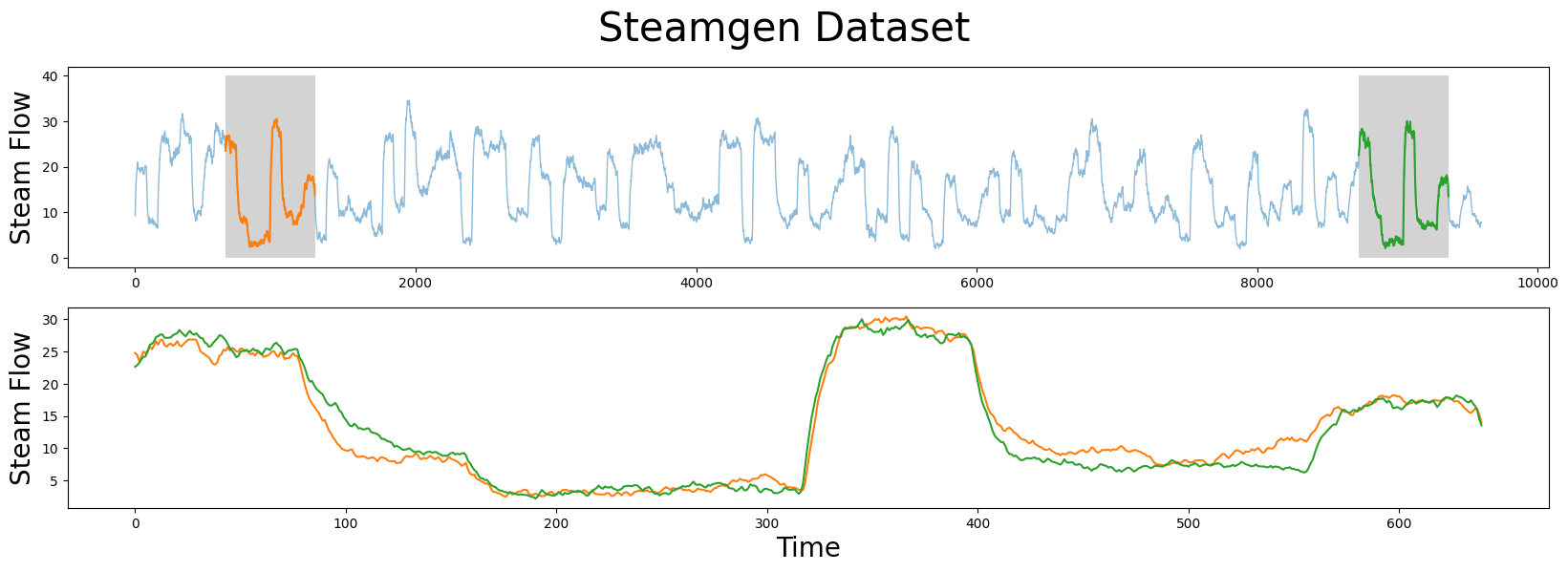
这些数据是使用模糊模型生成的,旨在模拟位于伊利诺伊州香槟的阿博特发电厂的蒸汽发生器。我们感兴趣的数据特征是输出蒸汽流量的遥测,单位为kg/s,数据每三秒“采样”一次,总共有9,600个数据点。
我们正在寻找的图案(模式)在下面突出显示,但仍然很难确定橙色和绿色子序列是否匹配,也就是说,直到我们放大它们并将子序列重叠在一起。现在,我们可以清楚地看到该图案非常相似!
m = 640
fig, axs = plt.subplots(2)
plt.suptitle('Steamgen Dataset', fontsize='30')
axs[0].set_ylabel("Steam Flow", fontsize='20')
axs[0].plot(steam_df['steam flow'], alpha=0.5, linewidth=1)
axs[0].plot(steam_df['steam flow'].iloc[643:643+m])
axs[0].plot(steam_df['steam flow'].iloc[8724:8724+m])
rect = Rectangle((643, 0), m, 40, facecolor='lightgrey')
axs[0].add_patch(rect)
rect = Rectangle((8724, 0), m, 40, facecolor='lightgrey')
axs[0].add_patch(rect)
axs[1].set_xlabel("Time", fontsize='20')
axs[1].set_ylabel("Steam Flow", fontsize='20')
axs[1].plot(steam_df['steam flow'].values[643:643+m], color='C1')
axs[1].plot(steam_df['steam flow'].values[8724:8724+m], color='C2')
plt.show()
使用 STUMPI#
现在,让我们看看当我们用前2000个数据点初始化我们的 stumpy.stumpi 时矩阵轮廓会发生什么:
T_full = steam_df['steam flow'].values
T_stream = T_full[:2000]
stream = stumpy.stumpi(T_stream, m, egress=False) # Don't egress/remove the oldest data point when streaming
然后逐步添加一个新的数据点并更新我们的结果:
windows = [(stream.P_, T_stream)]
P_max = -1
for i in range(2000, len(T_full)):
t = T_full[i]
stream.update(t)
if i % 50 == 0:
windows.append((stream.P_, T_full[:i+1]))
if stream.P_.max() > P_max:
P_max = stream.P_.max()
当我们绘制成长时间序列(上图), T_stream,以及矩阵剖面(下图), P,我们可以观察到随着新数据的添加矩阵剖面的演变:
fig, axs = plt.subplots(2, sharex=True, gridspec_kw={'hspace': 0})
rect = Rectangle((643, 0), m, 40, facecolor='lightgrey')
axs[0].add_patch(rect)
rect = Rectangle((8724, 0), m, 40, facecolor='lightgrey')
axs[0].add_patch(rect)
axs[0].set_xlim((0, T_full.shape[0]))
axs[0].set_ylim((-0.1, T_full.max()+5))
axs[1].set_xlim((0, T_full.shape[0]))
axs[1].set_ylim((-0.1, P_max+5))
axs[0].axvline(x=643, linestyle="dashed")
axs[0].axvline(x=8724, linestyle="dashed")
axs[1].axvline(x=643, linestyle="dashed")
axs[1].axvline(x=8724, linestyle="dashed")
axs[0].set_ylabel("Steam Flow", fontsize='20')
axs[1].set_ylabel("Matrix Profile", fontsize='20')
axs[1].set_xlabel("Time", fontsize='20')
lines = []
for ax in axs:
line, = ax.plot([], [], lw=2)
lines.append(line)
line, = axs[1].plot([], [], lw=2)
lines.append(line)
def init():
for line in lines:
line.set_data([], [])
return lines
def animate(window):
P, T = window
for line, data in zip(lines, [T, P]):
line.set_data(np.arange(data.shape[0]), data)
return lines
anim = animation.FuncAnimation(fig, animate, init_func=init,
frames=windows, interval=100,
blit=True, repeat=False)
anim_out = anim.to_jshtml()
plt.close() # Prevents duplicate image from displaying
if os.path.exists("None0000000.png"):
os.remove("None0000000.png") # Delete rogue temp file
HTML(anim_out)
# anim.save('/tmp/stumpi.mp4')