STUMPY 基础#
![]()
使用 STUMP 分析模式和异常#
本教程利用了研究论文的主要内容: Matrix Profile I & Matrix Profile II。
为了探索基本概念,我们将使用主要的 stump 函数来找到有趣的主题(模式)或异常(异常/新奇),并用两个不同的时间序列数据集来演示这些概念:
Steamgen 数据集
纽约市出租车乘客数据集
stump 是流行的 STOMP 算法的 Numba JIT 编译版本,该算法在原始 Matrix Profile II 论文中有详细描述。 stump 能够进行并行计算,并在指定时间序列中对模式和异常值执行有序搜索,并利用某些计算的局部性来最小化运行时间。
开始使用#
让我们导入需要加载、分析和绘制数据的包。
%matplotlib inline

import pandas as pd
import stumpy
import numpy as np
import matplotlib.pyplot as plt
import matplotlib.dates as dates
from matplotlib.patches import Rectangle
import datetime as dt

plt.style.use('https://raw.githubusercontent.com/TDAmeritrade/stumpy/main/docs/stumpy.mplstyle')
什么是图样?#
时间序列模式是指在较长时间序列中大致重复的子序列。能够说一个子序列“近似重复”需要你能够相互比较子序列。在STUMPY的情况下,时间序列中的所有子序列可以通过计算成对的z标准化欧氏距离进行比较,然后仅存储其最近邻的索引。这个最近邻距离向量被称为matrix profile,而时间序列中每个最近邻的索引被称为matrix profile index。幸运的是,stump函数接受任何时间序列(具有浮点值)并计算矩阵配置文件及其索引,从而可以立即找到时间序列模式。让我们看一个例子:
加载Steamgen数据集#
这些数据是使用模糊模型生成的,旨在模拟位于伊利诺伊州香槟的阿博特发电厂的蒸汽发生器。我们感兴趣的数据特征是输出蒸汽流量的遥测,单位为kg/s,数据每三秒“采样”一次,总共有9,600个数据点。
steam_df = pd.read_csv("https://zenodo.org/record/4273921/files/STUMPY_Basics_steamgen.csv?download=1")
steam_df.head()
| 鼓压力 | 过剩氧气 | 水位 | 蒸汽流量 | |
|---|---|---|---|---|
| 0 | 320.08239 | 2.506774 | 0.032701 | 9.302970 |
| 1 | 321.71099 | 2.545908 | 0.284799 | 9.662621 |
| 2 | 320.91331 | 2.360562 | 0.203652 | 10.990955 |
| 3 | 325.00252 | 0.027054 | 0.326187 | 12.430107 |
| 4 | 326.65276 | 0.285649 | 0.753776 | 13.681666 |
可视化Steamgen数据集#
plt.suptitle('Steamgen Dataset', fontsize='30')
plt.xlabel('Time', fontsize ='20')
plt.ylabel('Steam Flow', fontsize='20')
plt.plot(steam_df['steam flow'].values)
plt.show()
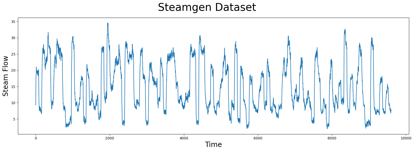
花一点时间仔细用肉眼观察上面的图表。如果有人告诉你有一个大致重复的模式,你能发现它吗?即使对于计算机来说,这也可能非常具有挑战性。你应该寻找的内容如下:
手动查找模式#
m = 640
fig, axs = plt.subplots(2)
plt.suptitle('Steamgen Dataset', fontsize='30')
axs[0].set_ylabel("Steam Flow", fontsize='20')
axs[0].plot(steam_df['steam flow'], alpha=0.5, linewidth=1)
axs[0].plot(steam_df['steam flow'].iloc[643:643+m])
axs[0].plot(steam_df['steam flow'].iloc[8724:8724+m])
rect = Rectangle((643, 0), m, 40, facecolor='lightgrey')
axs[0].add_patch(rect)
rect = Rectangle((8724, 0), m, 40, facecolor='lightgrey')
axs[0].add_patch(rect)
axs[1].set_xlabel("Time", fontsize='20')
axs[1].set_ylabel("Steam Flow", fontsize='20')
axs[1].plot(steam_df['steam flow'].values[643:643+m], color='C1')
axs[1].plot(steam_df['steam flow'].values[8724:8724+m], color='C2')
plt.show()
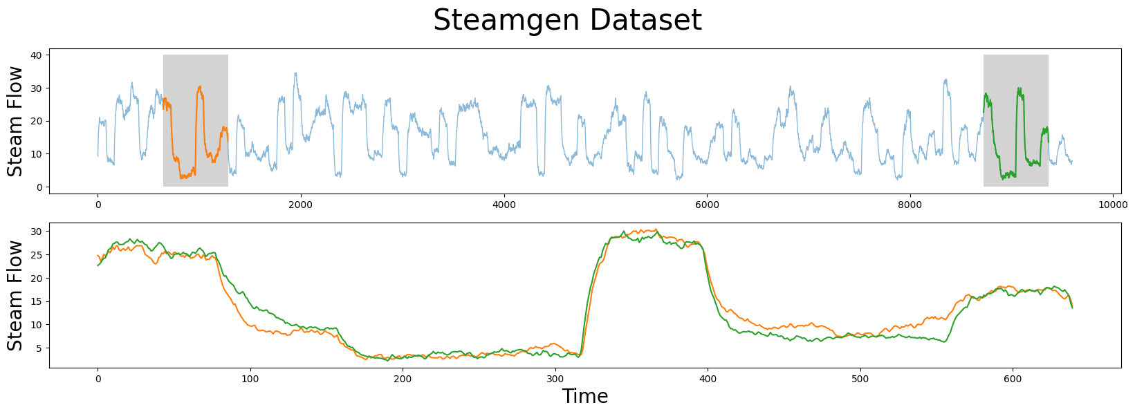
我们正在寻找的模式在上面被突出显示,但仍然很难确定橙色和绿色子序列是否匹配(上面面板),也就是说,直到我们放大它们并将子序列叠加在一起(下面面板)。现在,我们可以清楚地看到模式非常相似!计算矩阵剖面的基本价值在于,它不仅允许你快速找到模式,还能识别时间序列中所有子序列的最近邻。请注意,我们实际上并没有做任何特别的事情来定位模式,只是从原始论文中获取位置并绘制它们。现在,让我们使用我们的steamgen数据并对其应用stump函数:
使用STUMP查找模式#
m = 640
mp = stumpy.stump(steam_df['steam flow'], m)
stump 需要两个参数:
时间序列
一个窗口大小,
m
在这种情况下,基于一些领域专业知识,我们选择了 m = 640,这大致相当于半小时的窗口。同样, stump 的输出是一个数组,包含所有矩阵轮廓值(即,z-标准化的欧几里得距离到你的最近邻居)以及矩阵轮廓索引,分别在第一和第二列(我们暂时忽略第三列和第四列)。要识别该主题的索引位置,我们需要找到矩阵轮廓 mp[:, 0] 具有最小值的索引位置:
motif_idx = np.argsort(mp[:, 0])[0]

print(f"The motif is located at index {motif_idx}")
The motif is located at index 643
有了这个 motif_idx 信息,我们还可以通过交叉引用矩阵轮廓索引来确定其最近邻的位置, mp[:, 1]:
nearest_neighbor_idx = mp[motif_idx, 1]

print(f"The nearest neighbor is located at index {nearest_neighbor_idx}")
The nearest neighbor is located at index 8724
现在,让我们将所有这些结合在一起,并将矩阵剖面绘制在原始数据旁边:
fig, axs = plt.subplots(2, sharex=True, gridspec_kw={'hspace': 0})
plt.suptitle('Motif (Pattern) Discovery', fontsize='30')

axs[0].plot(steam_df['steam flow'].values)
axs[0].set_ylabel('Steam Flow', fontsize='20')
rect = Rectangle((motif_idx, 0), m, 40, facecolor='lightgrey')
axs[0].add_patch(rect)
rect = Rectangle((nearest_neighbor_idx, 0), m, 40, facecolor='lightgrey')
axs[0].add_patch(rect)
axs[1].set_xlabel('Time', fontsize ='20')
axs[1].set_ylabel('Matrix Profile', fontsize='20')
axs[1].axvline(x=motif_idx, linestyle="dashed")
axs[1].axvline(x=nearest_neighbor_idx, linestyle="dashed")
axs[1].plot(mp[:, 0])
plt.show()
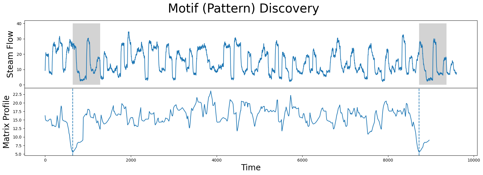
我们学到的是,矩阵轮廓中的全局最小值(垂直虚线)对应于构成模式对的两个子序列的位置!这两个子序列之间的确切z标准化欧几里得距离为:
mp[motif_idx, 0]
5.491619827769537
在STUMPY版本1.12.0之后添加
可以通过 P_ 属性直接访问矩阵谱距离,通过 I_ 属性访问矩阵谱索引:
mp = stumpy.stump(T, m)
print(mp.P_, mp.I_)  # print the matrix profile and the matrix profile indices
此外,左侧和右侧矩阵轮廓索引还可以通过 left_I_ 和 right_I_ 属性分别访问。
因此,这个距离不是零,因为我们看到两个子序列并不是完全匹配的,但是,相对于矩阵轮廓的其余部分(即,与均值或中位数矩阵轮廓值相比),我们可以理解这个模式是一个显著好的匹配。
使用 STUMP 查找潜在异常(不和谐)#
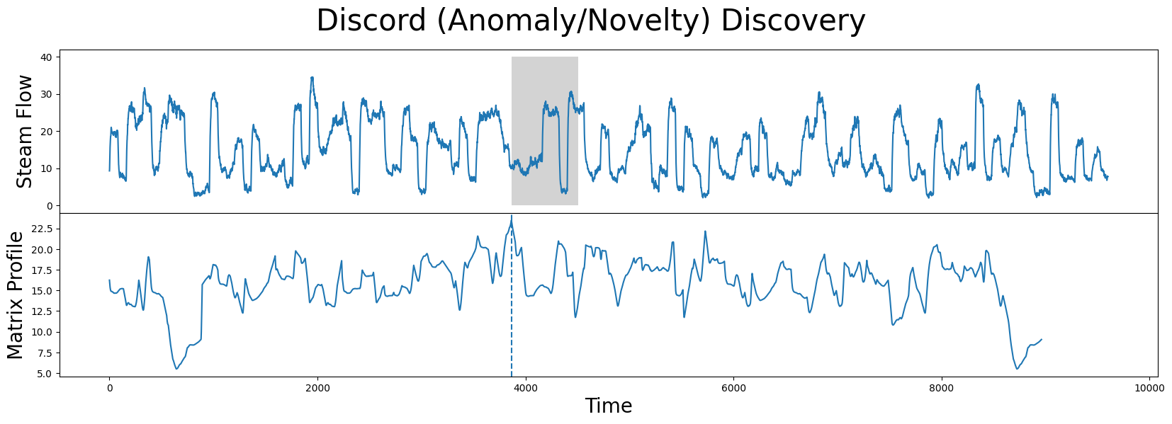
相反,在我们矩阵剖面中具有最大值的位置索引(从 stump 计算得出)是:
discord_idx = np.argsort(mp[:, 0])[-1]

print(f"The discord is located at index {discord_idx}")
The discord is located at index 3864
而这个不和谐的最近邻距离相当远:
nearest_neighbor_distance = mp[discord_idx, 0]

print(f"The nearest neighbor subsequence to this discord is {nearest_neighbor_distance} units away")
The nearest neighbor subsequence to this discord is 23.47616836730202 units away
位于该全局最大值的子序列也称为不和谐、创新或“潜在异常”:
fig, axs = plt.subplots(2, sharex=True, gridspec_kw={'hspace': 0})
plt.suptitle('Discord (Anomaly/Novelty) Discovery', fontsize='30')

axs[0].plot(steam_df['steam flow'].values)
axs[0].set_ylabel('Steam Flow', fontsize='20')
rect = Rectangle((discord_idx, 0), m, 40, facecolor='lightgrey')
axs[0].add_patch(rect)
axs[1].set_xlabel('Time', fontsize ='20')
axs[1].set_ylabel('Matrix Profile', fontsize='20')
axs[1].axvline(x=discord_idx, linestyle="dashed")
axs[1].plot(mp[:, 0])
plt.show()
现在您已经掌握了STUMPY的基本知识,并理解如何从时间序列中发现模式和异常,我们将留给您去研究steamgen数据集中其他有趣的局部最小值和局部最大值。
为了进一步发展/增强我们日益增长的直觉,让我们继续探索另一个数据集!
加载纽约市出租车乘客数据集#
首先,我们将下载历史数据,该数据表示2014年秋季75天内纽约市出租车乘客数量的半小时平均值。
我们提取这些数据并将其插入到一个 pandas 数据框中,确保时间戳存储为 datetime 对象,值为 float64 类型。请注意,我们将进行一些额外的数据清理,以便您可以看到一个包含时间戳的示例。但请注意,stump 在计算矩阵剖面时实际上并不使用或需要时间戳列。
taxi_df = pd.read_csv("https://zenodo.org/record/4276428/files/STUMPY_Basics_Taxi.csv?download=1")
taxi_df['value'] = taxi_df['value'].astype(np.float64)
taxi_df['timestamp'] = pd.to_datetime(taxi_df['timestamp'], errors='ignore')
taxi_df.head()
/tmp/ipykernel_797/748043925.py:3: FutureWarning: errors='ignore' is deprecated and will raise in a future version. Use to_datetime without passing `errors` and catch exceptions explicitly instead
  taxi_df['timestamp'] = pd.to_datetime(taxi_df['timestamp'], errors='ignore')
/tmp/ipykernel_797/748043925.py:3: UserWarning: Could not infer format, so each element will be parsed individually, falling back to `dateutil`. To ensure parsing is consistent and as-expected, please specify a format.
  taxi_df['timestamp'] = pd.to_datetime(taxi_df['timestamp'], errors='ignore')
| 时间戳 | 值 | |
|---|---|---|
| 0 | 2014-10-01 00:00:00 | 12751.0 |
| 1 | 2014-10-01 00:30:00 | 8767.0 |
| 2 | 2014-10-01 01:00:00 | 7005.0 |
| 3 | 2014-10-01 01:30:00 | 5257.0 |
| 4 | 2014-10-01 02:00:00 | 4189.0 |
可视化出租车数据集#
# This code is going to be utilized to control the axis labeling of the plots
DAY_MULTIPLIER = 7  # Specify for the amount of days you want between each labeled x-axis tick

x_axis_labels = taxi_df[(taxi_df.timestamp.dt.hour==0)]['timestamp'].dt.strftime('%b %d').values[::DAY_MULTIPLIER]
x_axis_labels[1::2] = " "
x_axis_labels, DAY_MULTIPLIER

plt.suptitle('Taxi Passenger Raw Data', fontsize='30')
plt.xlabel('Window Start Date', fontsize ='20')
plt.ylabel('Half-Hourly Average\nNumber of Taxi Passengers', fontsize='20')
plt.plot(taxi_df['value'])

plt.xticks(np.arange(0, taxi_df['value'].shape[0], (48*DAY_MULTIPLIER)/2), x_axis_labels)
plt.xticks(rotation=75)
plt.minorticks_on()
plt.margins(x=0)
plt.show()
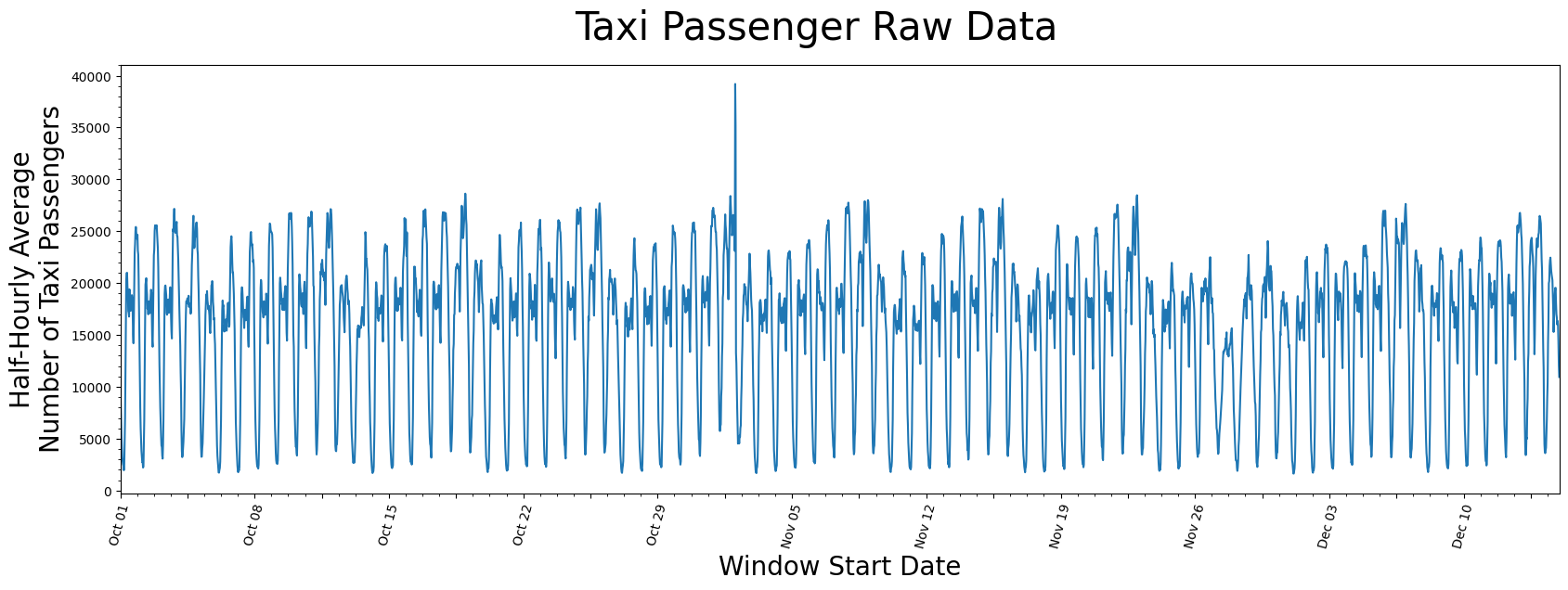
看起来1天和7天之间存在一般的周期性,这可能可以通过这样的事实来解释:白天使用出租车的人比晚上多,并且可以合理地说,大多数周的出租车乘客模式相似。此外,可能在10月底附近窗口右侧有一个异常值,但除此之外,仅仅通过观察原始数据无法得出任何结论。
生成矩阵轮廓#
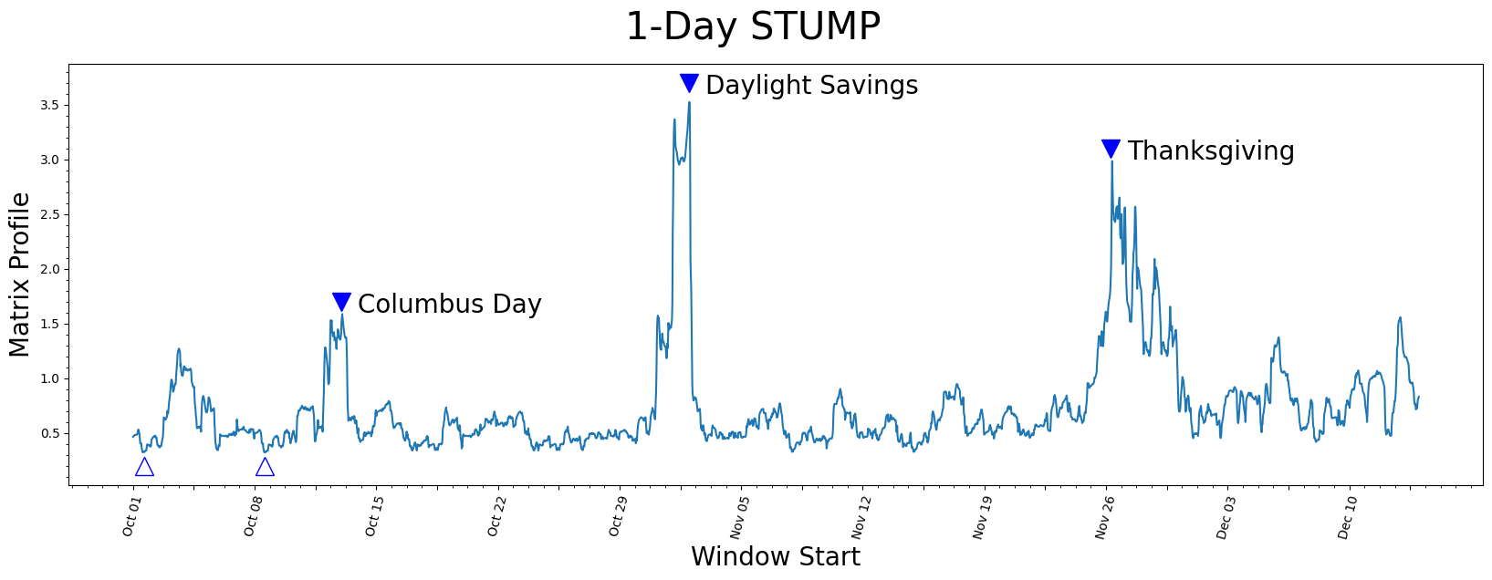
再次定义窗口大小 m 通常需要一定程度的领域知识,但我们稍后将演示 stump 对此参数的变化具有鲁棒性。由于这些数据是每半小时采集一次,我们选择一个值 m = 48 来表示恰好一天的时间跨度:
m = 48
mp = stumpy.stump(taxi_df['value'], m=m)
可视化矩阵轮廓#
plt.suptitle('1-Day STUMP', fontsize='30')
plt.xlabel('Window Start', fontsize ='20')
plt.ylabel('Matrix Profile', fontsize='20')
plt.plot(mp[:, 0])

plt.plot(575, 1.7, marker="v", markersize=15, color='b')
plt.text(620, 1.6, 'Columbus Day', color="black", fontsize=20)
plt.plot(1535, 3.7, marker="v", markersize=15, color='b')
plt.text(1580, 3.6, 'Daylight Savings', color="black", fontsize=20)
plt.plot(2700, 3.1, marker="v", markersize=15, color='b')
plt.text(2745, 3.0, 'Thanksgiving', color="black", fontsize=20)
plt.plot(30, .2, marker="^", markersize=15, color='b', fillstyle='none')
plt.plot(363, .2, marker="^", markersize=15, color='b', fillstyle='none')
plt.xticks(np.arange(0, 3553, (m*DAY_MULTIPLIER)/2), x_axis_labels)
plt.xticks(rotation=75)
plt.minorticks_on()
plt.show()
理解矩阵特征#
让我们来理解一下我们正在看什么。
最低值#
最低值(开口三角形)被认为是一种特征,因为它们表示具有最小z标准化欧几里得距离的最近邻子序列对。有趣的是,两个最低数据点恰好相隔7天,这表明,在这个数据集中,除了更明显的每日周期性之外,可能还有七天的周期性。
最高值#
那么,最高的矩阵剖面值(填充三角形)怎么样呢?具有最高(局部)值的子序列确实强调了它们的独特性。我们发现前三个峰恰好分别对应于哥伦布日、夏令时和感恩节的时间。
不同的窗口大小#
正如我们上面提到的,stump 应该对窗口大小参数 m 的选择具有鲁棒性。下面,我们通过使用不同窗口大小运行 stump 来演示操纵窗口大小对您得到的矩阵轮廓几乎没有影响。
days_dict ={
  "Half-Day": 24,
  "1-Day": 48,
  "2-Days": 96,
  "5-Days": 240,
  "7-Days": 336,
}

days_df = pd.DataFrame.from_dict(days_dict, orient='index', columns=['m'])
days_df.head()
| 米 | |
|---|---|
| 半天 | 24 |
| 1天 | 48 |
| 2天 | 96 |
| 5天 | 240 |
| 7天 | 336 |
我们故意选择了对应人类可以选择的合理直观日长的时间段。
fig, axs = plt.subplots(5, sharex=True, gridspec_kw={'hspace': 0})
fig.text(0.5, -0.1, 'Subsequence Start Date', ha='center', fontsize='20')
fig.text(0.08, 0.5, 'Matrix Profile', va='center', rotation='vertical', fontsize='20')
for i, varying_m in enumerate(days_df['m'].values):
    mp = stumpy.stump(taxi_df['value'], varying_m)
    axs[i].plot(mp[:, 0])
    axs[i].set_ylim(0,9.5)
    axs[i].set_xlim(0,3600)
    title = f"m = {varying_m}"
    axs[i].set_title(title, fontsize=20, y=.5)
plt.xticks(np.arange(0, taxi_df.shape[0], (48*DAY_MULTIPLIER)/2), x_axis_labels)
plt.xticks(rotation=75)
plt.suptitle('STUMP with Varying Window Sizes', fontsize='30')
plt.show()
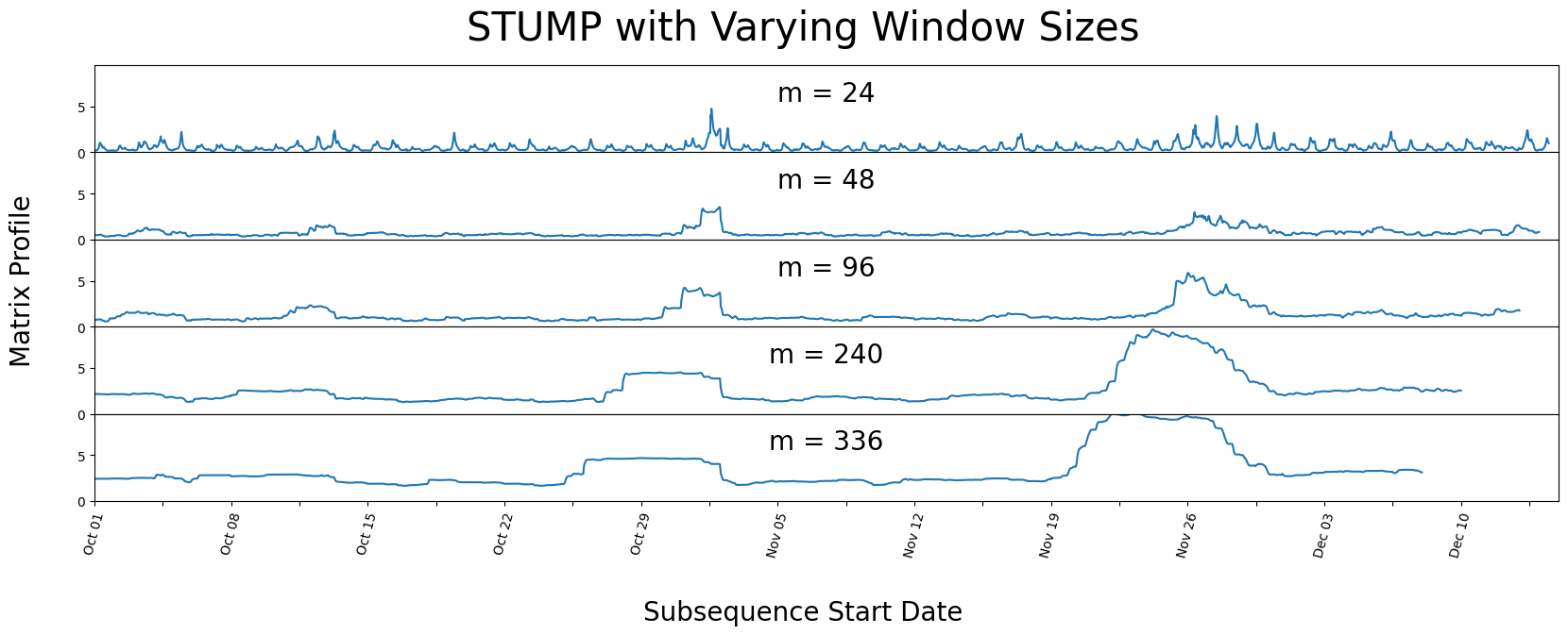
我们可以看到,即使在不同的窗口大小下,我们的峰值仍然显著。但看起来所有非峰值的值都在相互汇聚。这就是在运行 stump 之前了解数据上下文的重要性,因为拥有一个可能捕捉到数据集中重复模式或异常的窗口大小是有帮助的。
GPU-STUMP - 使用GPU加速的STUMP#
当你的时间序列中有几千个数据点时,你可能需要加速来帮助分析你的数据。幸运的是,你可以尝试 gpu_stump,这是一种超级快速的GPU加速替代方案,与 stump 相比,提供几百个CPU的速度,并且输出与 stump 相同:
import stumpy

mp = stumpy.gpu_stump(df['value'], m=m)  # Note that you'll need a properly configured NVIDIA GPU for this
实际上,如果您没有处理PII/SII数据,那么您可以尝试使用 gpu_stump 通过 这个Google Colab笔记。
困惑 - 分布式STUMP#
另外,如果您只能访问一组 CPU,并且您的数据需要保留在防火墙后,那么 stump 和 gpu_stump 可能不足以满足您的需求。相反,您可以尝试 stumped,这是一个依赖于 Dask distributed 的 stump 的分布式和并行实现:
import stumpy
from dask.distributed import Client

if __name__ == "__main__":
    with Client() as dask_client:
        mp = stumpy.stumped(dask_client, df['value'], m=m)  # Note that a dask client is needed
奖金部分#
理解矩阵轮廓的列输出#
对于任何一维时间序列, T,它的矩阵分析 mp,从 stumpy.stump(T, m) 计算得出,将包含4个明确的列,我们将在稍后进行描述。隐式地, mp 数组的第 i 行对应于为特定子序列 T[i : i + m] 计算的(4个)最近邻值的集合。
mp 的第一列包含矩阵特征(最近邻距离)值,P(请注意,由于零基索引,“第一列”的列索引值为零)。第二列包含(零基)索引位置,I,指示(上述)最近邻在 T 上的位置(请注意,任何负索引值都是“不良”值,表示无法找到最近邻)。
因此,对于第 i 个子序列 T[i : i + m],其最近邻(位于 T 的某个位置)具有起始索引位置 I = mp[i, 1],并且假设 I >= 0,这对应于在 T[I : I + m] 中找到的子序列。而第 i 个子序列的矩阵剖面值 P = [i, 0] 是 T[i : i + m] 和 T[I : I + m] 之间的确切(z标准化的欧几里得)距离。请注意,最近邻索引位置 I 可以位于任意位置。也就是说,依赖于第 i 个子序列,其最近邻 I 可以位于 i 之前/左侧(即 I <= i),或位于 i 之后/右侧(即 I >= i)。换句话说,对于最近邻的位置没有限制。然而,有时您可能希望只知道位于 i 之前/之后的最近邻,这就是 mp 的第 3 列和第 4 列的作用。
第三列包含“左”最近邻居沿T的位置索引,IL(以零为基准)。这里有一个约束条件,即IL < i或者IL必须在i之前/左侧。因此,i子序列的“左最近邻居”位于IL = mp[i, 2],对应于T[IL : IL + m]。
第四列包含“右”最近邻居沿T的位置索引,IR(以零为基准)。这里有一个约束条件,即IR > i或者IR必须在i之后/右侧。因此,i子序列的“右最近邻居”位于IR = mp[i, 3],对应于T[IR : IR + m]。
再者,请注意,任何负索引值都是“坏”值,表示无法找到最近邻。
为了更具体地加强这一点,让我们使用以下 mp 数组作为示例:
array([[1.626257115121311,  202, -1,  202],
       [1.7138456780667977,  65,  0,   65],
       [1.880293454724256,   66,  0,   66],
       [1.796922109741226,   67,  0,   67],
       [1.4943082939628236,  11,  1,   11],
       [1.4504278114808016,  12,  2,   12],
       [1.6294354134867932,  19,  0,   19],
       [1.5349365731102185, 229,  0,  229],
       [1.3930265554289831, 186,  1,  186],
       [1.5265881687159586, 187,  2,  187],
       [1.8022253384245739,  33,  3,   33],
       [1.4943082939628236,   4,  4,  118],
       [1.4504278114808016,   5,  5,  137],
       [1.680920620705546,  201,  6,  201],
       [1.5625058007723722, 237,  8,  237],
       [1.2860008417613522,  66,  9,   -1]]
这里,i = 0 处的子序列对应于 T[0 : 0 + m] 子序列,并且该子序列的最近邻位于 I = 202 (即,mp[0, 1])并对应于 T[202 : 202 + m] 子序列。T[0 : 0 + m] 和 T[202 : 202 + m] 之间的 z 归一化欧几里得距离实际上是 P = 1.626257115121311 (即,mp[0, 0])。接下来,注意左侧最近邻的位置是 IL = -1 (即,mp[0, 2]),由于负索引是“坏的”,这告诉我们无法找到左侧最近邻。希望这有意义,因为 T[0 : 0 + m] 是 T 中的第一个子序列,并且左侧不可能存在其他子序列!相反,右侧最近邻的位置是 IR = 202 (即,mp[0, 3])并对应于 T[202 : 202 + m] 子序列。
此外,在 i = 5 的子序列将对应于 T[5 : 5 + m] 子序列,而该子序列的最近邻位于 I = 12(即 mp[5, 1]),并对应于 T[12 : 12 + m] 子序列。T[5 : 5 + m] 和 T[12 : 12 + m] 之间的 z 标准化欧几里得距离实际上是 P = 1.4504278114808016(即 mp[5, 0])。接下来,左边最近邻的位置是 IL = 2(即 mp[5, 2]),并对应于 T[2 : 2 + m]。相反,右边最近邻的位置是 IR = 12(即 mp[5, 3]),并对应于 T[12 : 12 + m] 子序列。
同样,所有其他子序列都可以使用这种方法进行评估和解释!
寻找前K个模式#
现在您已经计算了时间序列的矩阵轮廓, mp,并识别出了最佳全局动机,您可能对在数据中发现其他动机感兴趣。然而,您会立即了解到,像 top_10_motifs_idx = np.argsort(mp[:, 0])[10] 这样的操作并不能得到您想要的结果,因为这仅返回可能接近全局动机的索引位置!相反,在识别出最佳动机(即,具有最小值的矩阵轮廓位置)后,您需要首先排除围绕动机对的局部区域(即,排除区),方法是将它们的矩阵轮廓值设置为 np.inf,然后再搜索下一个动机。然后,您需要对每个后续动机重复“排除和搜索”过程。幸运的是,STUMPY提供了两个附加函数,即 stumpy.motifs 和 stumpy.match,可以帮助简化这个过程。虽然这超出了本基础教程的范围,但我们鼓励您去了解它们!
总结#
就这样!您现在已经加载了一个数据集,通过我们的包使用stump运行,并能够提取出两个不同时间序列中存在的多个模式和异常的结论。您现在可以导入这个包并在自己的项目中使用。祝您编码愉快!