形状发现#
![]()
本教程探讨了来自研究论文的“Shapelet Discovery”案例研究: The Swiss Army Knife of Time Series Data Mining: Ten Useful Things You Can Do with the Matrix Profile and Ten Lines of Code” (见第3.7节)。此外,您可能还想参考 Matrix Profile I 和 Time Series Shapelets: A New Primitive for Data Mining 论文,以获取更多信息和其他相关示例。
什么是形状元?#
非正式地说,时间序列“形状体”是时间序列的子序列,从某种意义上讲,它们是一个类别的最大代表。例如,想象一下,如果你有一个时间序列,它跟踪你家中大型电器每秒钟使用的电力消耗,持续了五年。每当你运行烘干机、洗碗机或空调时,你的电表会记录消耗的电力,仅通过查看时间序列,你很可能能够将每个电器关联到一个电力消耗“特征”(即形状、持续时间、最大能量使用等)。这些模式可能是明显的或微妙的,正是它们独特的“形状”的时间序列子序列使你能够区分每个电器类别。因此,这些所谓的形状体可能对于分类包含形状体出现的未标记时间序列是有用的。如果这听起来有点术语化,不用担心,希望通过下面的例子一切会变得更清晰。
最近的研究(见上文)表明,矩阵剖面可以有效地识别特定类别的形状,因此在本教程中,我们将基于我们的矩阵剖面知识,演示如何使用 STUMPY 轻松发现有趣的形状,只需几行附加代码。
开始使用#
让我们导入我们需要的包,以加载、分析和绘制数据,随后,构建简单的决策树模型。
%matplotlib inline

import stumpy
import pandas as pd
import numpy as np
import matplotlib.pyplot as plt
from sklearn import tree
from sklearn import metrics

plt.style.use('https://raw.githubusercontent.com/TDAmeritrade/stumpy/main/docs/stumpy.mplstyle')
加载GunPoint数据集#
这个数据集是一个动作捕捉时间序列,跟踪演员的右手运动,并包含两个类别:
GunPoint
在Gun类中,演员们从臀部挂着的枪套中抽出一把真实的手枪,将手枪对准目标约一秒钟,然后将手枪放回枪套,双手放松在身体两侧。在Point类中,演员们将手枪放在身体侧面,而是用食指指向目标(即没有手枪)约一秒钟,然后将双手放回身体两侧。对于这两个类,演员的右手质心被追踪以表示其运动。
下面,我们将提取原始数据,将其分为 gun_df 和 point_df,然后,对于每个相应的类,将所有单独的样本连接成一个长的时间序列。此外,我们通过在每个样本后附加一个 NaN 值来建立每个样本的明确边界(即样本开始和结束的地方)。这有助于确保所有矩阵轮廓计算不会返回跨越多个样本的人工子序列:
train_df = pd.read_csv("https://zenodo.org/record/4281349/files/gun_point_train_data.csv?download=1")

gun_df = train_df[train_df['0'] == 0].iloc[:, 1:].reset_index(drop=True)
gun_df = (gun_df.assign(NaN=np.nan)
                .stack(dropna=False).to_frame().reset_index(drop=True)
                .rename({0: "Centroid Location"}, axis='columns')
         )

point_df = train_df[train_df['0'] == 1].iloc[:, 1:].reset_index(drop=True)
point_df = (point_df.assign(NaN=np.nan)
                    .stack(dropna=False).to_frame().reset_index(drop=True)
                    .rename({0: "Centroid Location"}, axis='columns')
           )
/tmp/ipykernel_843/3588988851.py:5: FutureWarning: The previous implementation of stack is deprecated and will be removed in a future version of pandas. See the What's New notes for pandas 2.1.0 for details. Specify future_stack=True to adopt the new implementation and silence this warning.
  .stack(dropna=False).to_frame().reset_index(drop=True)
/tmp/ipykernel_843/3588988851.py:11: FutureWarning: The previous implementation of stack is deprecated and will be removed in a future version of pandas. See the What's New notes for pandas 2.1.0 for details. Specify future_stack=True to adopt the new implementation and silence this warning.
  .stack(dropna=False).to_frame().reset_index(drop=True)
可视化GunPoint数据集#
接下来,让我们绘制数据并可视化在没有枪支和实际存在枪支时运动的差异:
fig, axs = plt.subplots(2, sharex=True, gridspec_kw={'hspace': 0})
plt.suptitle('Point vs. Gun', fontsize='30')
plt.xlabel('Time', fontsize ='20')
fig.text(0.09, 0.5, 'Centroid Location', va='center', rotation='vertical', fontsize='20')

axs[0].plot(point_df, label="Point")
axs[0].legend()

axs[1].plot(gun_df, color="C1", label="Gun")
axs[1].legend()

plt.show()
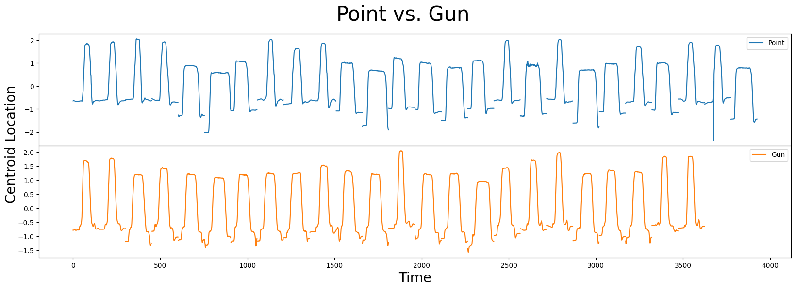
在这个数据集中,你会看到 Point 和 Gun 的样本分别为 26 和 24。两个类别都包含窄/宽样本和垂直移动的重心位置,这使得区分它们变得具有挑战性。你能识别出 Point 和 Gun 之间的任何细微差别(即,形状特征)吗,这可能帮助你区分这两个类别?
事实证明,矩阵剖面可能有助于我们自动识别潜在的形状特征!
通过矩阵剖面寻找候选形状#
从我们的 寻找两个时间序列之间的保守模式教程 中回忆到,从单个时间序列 \(T_A\) 计算出的矩阵轮廓 \(P_{AA}\) 被称为“自连接”,允许您识别 \(T_A\) 内部的保守子序列。然而,跨两个不同时间序列 \(T_A\) 和 \(T_B\) 计算的矩阵轮廓 \(P_{AB}\) 更常被称为“AB连接”。本质上,AB连接比较 \(T_A\) 中的所有子序列和 \(T_B\) 中的所有子序列,以确定 \(T_A\) 中是否存在也可以在 \(T_B\) 中找到的子序列。换句话说,生成的矩阵轮廓 \(P_{AB}\) 为 \(T_A\) 中的每个子序列标注其在 \(T_B\) 中最佳匹配的子序列。相反,如果我们交换时间序列并计算 \(P_{BA}\)(即“BA连接”),那么这将为 \(T_B\) 中的每个子序列标注其在 \(T_A\) 中的最近邻子序列。
根据Matrix Profile I论文的H部分,声称我们可以利用矩阵轮廓来启发式地“建议”候选形状子,主要直觉是,如果在Gun类中存在一个判别模式而在Point类中不存在(或反之),那么我们应该期望在它们相应的\(P_{Point,Point}\)、\(P_{Point,Gun}\)(或\(P_{Gun, Gun}\)、\(P_{Gun,Point}\))矩阵轮廓中看到一个或多个“峰值”,而高度的任何显著差异可能是良好候选形状子的强指标。
所以,首先,让我们计算矩阵剖面, \(P_{Point, Point}\)(自连接)和 \(P_{Point, Gun}\)(AB连接),为了简单起见,我们使用的子序列长度为 m = 38,这是为该数据集报告的最佳形状的长度:
m = 38
P_Point_Point = stumpy.stump(point_df["Centroid Location"], m)[:, 0].astype(float)
P_Point_Gun = stumpy.stump(point_df["Centroid Location"], m, gun_df["Centroid Location"], ignore_trivial=False)[:, 0].astype(float)
由于我们的时间序列中包含一些 np.nan 值,因此矩阵轮廓的输出将包含几个 np.inf 值。因此,我们将通过手动将它们转换为 np.nan 来进行调整:
P_Point_Point[P_Point_Point == np.inf] = np.nan
P_Point_Gun[P_Point_Gun == np.inf] = np.nan
现在我们将在彼此之上重叠绘制它们:
plt.plot(P_Point_Point, label="$P_{Point,Point}$")
plt.plot(P_Point_Gun, color="C1", label="$P_{Point,Gun}$")
plt.xlabel("Time", fontsize="20")
plt.ylabel("Matrix Profile", fontsize="20")
plt.legend()
plt.show()

接下来,我们可以通过绘制 \(P_{Point, Point}\) 和 \(P_{Point, Gun}\) 之间的差异来突出两个矩阵轮廓之间的主要偏差。 直观上, \(P_{Point, Point}\) 将小于 \(P_{Point, Gun}\),因为我们期望同一类别中的子序列比不同类别的子序列更相似:
P_diff = P_Point_Gun - P_Point_Point

idx = np.argpartition(np.nan_to_num(P_diff), -10)[-10:]  # get the top 10 peak locations in P_diff
plt.suptitle("", fontsize="30")
plt.xlabel("Time", fontsize="20")
plt.ylabel("$P_{diff} = P_{Point,Gun} - P_{Point, Point}$", fontsize="20")
plt.plot(idx, P_diff[idx], color="C1", marker="o", linewidth=0, markersize=10)
plt.plot(P_diff)
plt.show()
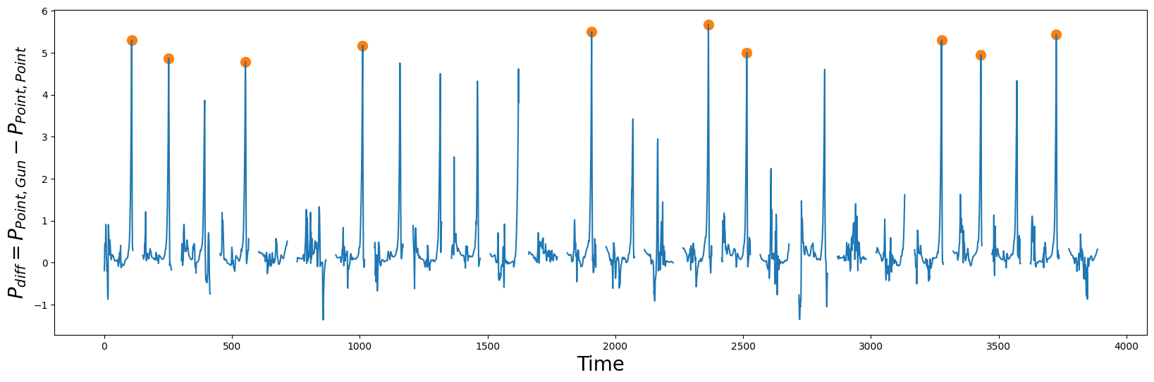
在 \(P_{diff}\) 中的峰值(橙色圆圈)是良好形状候选者的指标,因为它们表明在它们自身类别中模式保持良好(即 \(P_{Point,Point}\) 自连接),但与其他类别中的最近匹配(即 \(P_{Point, Gun}\) AB-连接)非常不同。掌握了这些知识,让我们提取发现的形状并绘制它们:
point_shapelets = []
for i in idx:
    shapelet = point_df.iloc[i : i + m, 0]
    point_shapelets.append(shapelet)

plt.xlabel("Time", fontsize="20")
plt.ylabel('Centroid Location', fontsize='20')
plt.plot(point_df, label="Point")
for i, shapelet in zip(idx, point_shapelets):
    plt.plot(range(i, i + m), shapelet, color="C1", linewidth=3.0)
plt.legend()
plt.show()
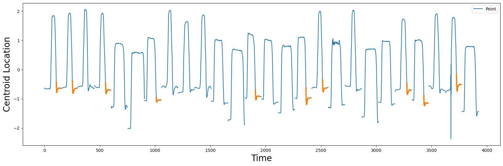
根据这些候选形状(橙色),两个类别之间主要的区分因素在于演员的手是如何将(假想的)枪归还到枪套中,然后在演员身旁放松的。根据原作者的说法,Point 类“有一个‘下沉’的地方,演员将手放在身旁,是惯性使她的手被带得有点太远,因此她被迫修正这一点——作者称之为‘过度射击’的现象。”
构建一个简单的分类器#
现在我们已经确定了10个候选形状,让我们基于这些形状构建10个独立的决策树模型,并看看它们能多好地帮助我们区分Point类和Gun类。幸运的是,数据集中包括一个训练集(上面)以及一个独立的测试集,我们可以使用这些来评估模型的准确性:
test_df = df = pd.read_csv("https://zenodo.org/record/4281349/files/gun_point_test_data.csv?download=1")

# Get the train and test targets
y_train = train_df.iloc[:, 0]
y_test = test_df.iloc[:, 0]
现在,对于我们的分类任务,每个形状需要根据其预测能力进行评估。因此,我们首先计算每个时间序列或样本中一个形状与每个子序列之间的距离轮廓(成对的欧几里得距离)。然后,保留最小值以了解是否在时间序列中找到了形状的接近匹配。stumpy.mass函数非常适合这个任务:
def distance_to_shapelet(data, shapelet):
    """
    Compute the minimum distance between each data sample and a shapelet of interest
    """
    data = np.asarray(data)
    X = np.empty(len(data))
    for i in range(len(data)):
        D = stumpy.mass(shapelet, data[i])
        X[i] = D.min()

    return X.reshape(-1, 1)
clf = tree.DecisionTreeClassifier()

for i, shapelet in enumerate(point_shapelets):
    X_train = distance_to_shapelet(train_df.iloc[:, 1:], shapelet)
    X_test = distance_to_shapelet(test_df.iloc[:, 1:], shapelet)
    clf.fit(X_train, y_train)
    y_pred = clf.predict(X_test.reshape(-1, 1))
    print(f"Accuracy for shapelet {i} = {round(metrics.accuracy_score(y_test, y_pred), 3)}")
Accuracy for shapelet 0 = 0.867
Accuracy for shapelet 1 = 0.833
Accuracy for shapelet 2 = 0.807
Accuracy for shapelet 3 = 0.833
Accuracy for shapelet 4 = 0.933
Accuracy for shapelet 5 = 0.873
Accuracy for shapelet 6 = 0.873
Accuracy for shapelet 7 = 0.833
Accuracy for shapelet 8 = 0.913
Accuracy for shapelet 9 = 0.86
如我们所见,所有的形状小样本都提供了一些合理的预测能力,有助于区分 Point 和 Gun 类别,但形状小样本 4 返回的准确率最高,为 93.3%,这个结果完全复现了 已发布的研究结果。太棒了!
奖励部分 - 第二类的形状#
作为额外的内容,我们还将从Gun时间序列中提取形状特征,以查看它们是否能为我们的模型增加任何额外的预测能力。该过程与我们上面解释的过程相同,只是我们专注于从gun_df派生的形状特征,因此我们在这里不会过多详细说明:
m = 38
P_Gun_Gun = stumpy.stump(gun_df["Centroid Location"], m)[:, 0].astype(float)
P_Gun_Point = stumpy.stump(gun_df["Centroid Location"], m, point_df["Centroid Location"], ignore_trivial=False)[:, 0].astype(float)
P_Gun_Gun[P_Gun_Gun == np.inf] = np.nan
P_Gun_Point[P_Gun_Point == np.inf] = np.nan
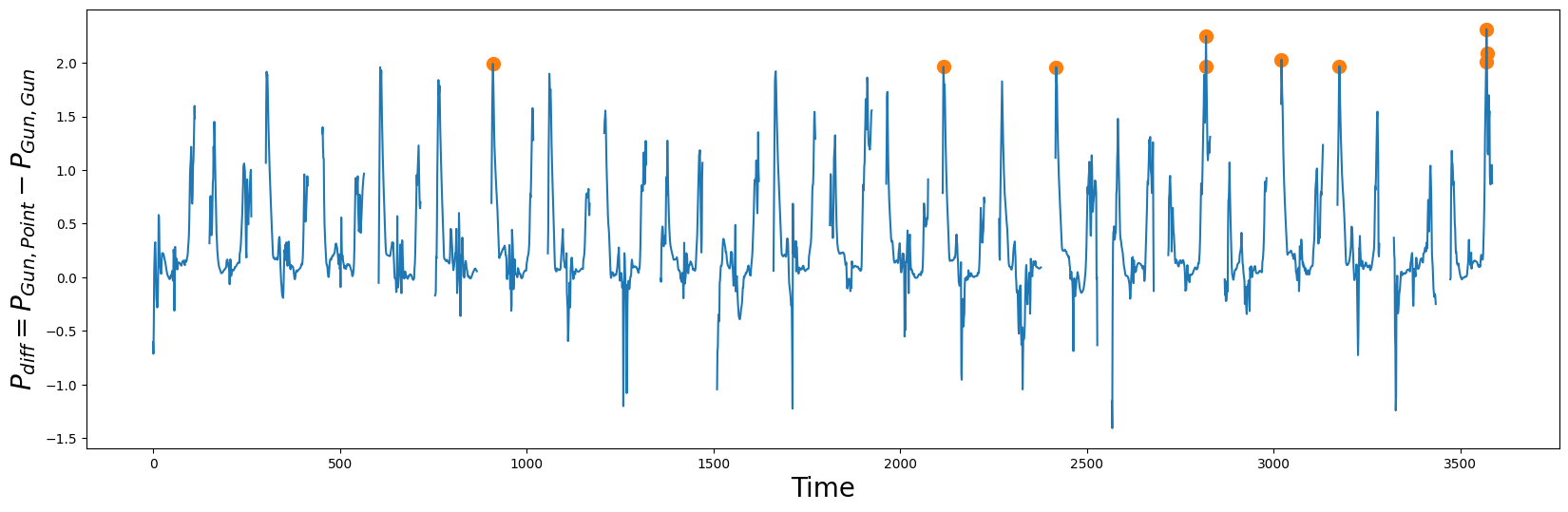
P_diff = P_Gun_Point - P_Gun_Gun
idx = np.argpartition(np.nan_to_num(P_diff), -10)[-10:] # get the top 10 peak locations in P_diff
plt.suptitle("", fontsize="30")
plt.xlabel("Time", fontsize="20")
plt.ylabel("$P_{diff} = P_{Gun, Point} - P_{Gun, Gun}$", fontsize="20")
plt.plot(idx, P_diff[idx], color="C1", marker="o", linewidth=0, markersize=10)
plt.plot(P_diff)
plt.show()
gun_shapelets = []
for i in idx:
    shapelet = gun_df.iloc[i : i + m, 0]
    gun_shapelets.append(shapelet)

plt.xlabel("Time", fontsize="20")
plt.ylabel('Centroid Location', fontsize='20')
plt.plot(gun_df, label="Gun")
for i, shapelet in zip(idx, gun_shapelets):
    plt.plot(range(i, i + m), shapelet, color="C1", linewidth=3.0)
plt.legend()
plt.show()

请注意,当物理枪存在时,在Gun绘制动作开始时发现的形状并不像Point样本那样平滑。同样,重新放回Gun似乎也需要一些微调。
最后,我们构建我们的模型,但这一次,我们结合了来自Gun形状特征和Point形状特征的距离特征:
clf = tree.DecisionTreeClassifier()

for i, (gun_shapelet, point_shapelet) in enumerate(zip(gun_shapelets, point_shapelets)):
    X_train_gun = distance_to_shapelet(train_df.iloc[:, 1:], gun_shapelet)
    X_train_point = distance_to_shapelet(train_df.iloc[:, 1:], point_shapelet)
    X_train = np.concatenate((X_train_gun, X_train_point), axis=1)
    X_test_gun = distance_to_shapelet(test_df.iloc[:, 1:], gun_shapelet)
    X_test_point = distance_to_shapelet(test_df.iloc[:, 1:], point_shapelet)
    X_test = np.concatenate((X_test_gun, X_test_point), axis=1)
    clf.fit(X_train, y_train)
    y_pred = clf.predict(X_test)
    print(f"Accuracy for shapelet {i} = {round(metrics.accuracy_score(y_test, y_pred), 3)}")
Accuracy for shapelet 0 = 0.913
Accuracy for shapelet 1 = 0.84
Accuracy for shapelet 2 = 0.82
Accuracy for shapelet 3 = 0.953
Accuracy for shapelet 4 = 0.933
Accuracy for shapelet 5 = 0.887
Accuracy for shapelet 6 = 0.913
Accuracy for shapelet 7 = 0.847
Accuracy for shapelet 8 = 0.913
Accuracy for shapelet 9 = 0.893
我们可以看到,如果我们同时包含来自Gun类shapelets和Point类shapelets的两个距离,分类器的准确率达到95.3%(Shapelet 3)!显然,添加来自第二类的距离也为模型提供了额外有用的信息。这是一个很好的结果,因为它的改进大约为2%。再次令人印象深刻的是,所有这些信息都可以通过利用矩阵轮廓“免费”提取。
总结#
就是这样!你刚刚学习了如何利用矩阵简介找到形状并用它们构建机器学习分类器。