Athey和Wager（2018）的二元处理策略学习器

本笔记本展示了Athey和Wager（2018）的政策学习器的CausalML实现的使用（https://arxiv.org/abs/1702.02896）。

%load_ext autoreload
%autoreload 2

import pandas as pd
import numpy as np
from matplotlib import pyplot as plt

from sklearn.model_selection import cross_val_predict, KFold
from sklearn.ensemble import GradientBoostingRegressor, GradientBoostingClassifier
from sklearn.tree import DecisionTreeClassifier

from causalml.optimize import PolicyLearner
from sklearn.tree import plot_tree
from lightgbm import LGBMRegressor
from causalml.inference.meta import BaseXRegressor

---------------------------------------------------------------------------
RuntimeError                              Traceback (most recent call last)
RuntimeError: module compiled against API version 0xe but this version of numpy is 0xd

The sklearn.utils.testing module is  deprecated in version 0.22 and will be removed in version 0.24. The corresponding classes / functions should instead be imported from sklearn.utils. Anything that cannot be imported from sklearn.utils is now part of the private API.

二元治疗策略学习

首先，我们生成一个具有二元处理的合成数据集。处理是在协变量条件下随机的。处理效果是异质的，对于某些个体来说是负面的。我们使用策略学习器将个体分类为处理/不处理组，以最大化总处理效果。

np.random.seed(1234)

n = 10000
p = 10

X = np.random.normal(size=(n, p))
ee = 1 / (1 + np.exp(X[:, 2]))
tt = 1 / (1 + np.exp(X[:, 0] + X[:, 1])/2) - 0.5
W = np.random.binomial(1, ee, n)
Y = X[:, 2] + W * tt + np.random.normal(size=n)

使用带有默认结果/处理估计器和简单策略分类器的策略学习器。

policy_learner = PolicyLearner(policy_learner=DecisionTreeClassifier(max_depth=2), calibration=True)

policy_learner.fit(X, W, Y)

PolicyLearner(model_mu=GradientBoostingRegressor(),
        model_w=GradientBoostingClassifier(),
\model_pi=DecisionTreeClassifier(max_depth=2))

plt.figure(figsize=(15,7))
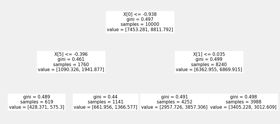
plot_tree(policy_learner.model_pi)

[Text(469.8, 340.2, 'X[0] <= -0.938\ngini = 0.497\nsamples = 10000\nvalue = [7453.281, 8811.792]'),
 Text(234.9, 204.12, 'X[5] <= -0.396\ngini = 0.461\nsamples = 1760\nvalue = [1090.326, 1941.877]'),
 Text(117.45, 68.03999999999996, 'gini = 0.489\nsamples = 619\nvalue = [428.371, 575.3]'),
 Text(352.35, 68.03999999999996, 'gini = 0.44\nsamples = 1141\nvalue = [661.956, 1366.577]'),
 Text(704.7, 204.12, 'X[1] <= 0.035\ngini = 0.499\nsamples = 8240\nvalue = [6362.955, 6869.915]'),
 Text(587.25, 68.03999999999996, 'gini = 0.491\nsamples = 4252\nvalue = [2957.726, 3857.306]'),
 Text(822.15, 68.03999999999996, 'gini = 0.498\nsamples = 3988\nvalue = [3405.228, 3012.609]')]

或者，可以直接从X-learner估计的ITE构建策略。

learner_x = BaseXRegressor(LGBMRegressor())
ite_x = learner_x.fit_predict(X=X, treatment=W, y=Y)

在这个例子中，策略学习器的表现优于基于ITE的策略，并接近真正的最优策略。

pd.DataFrame({
    'DR-DT Optimal': [np.mean((policy_learner.predict(X) + 1) * tt / 2)],
    'True Optimal': [np.mean((np.sign(tt) + 1) * tt / 2)],
    'X Learner': [
        np.mean((np.sign(ite_x) + 1) * tt / 2)
    ],
})

	DR-DT 最优	真实最优	X 学习器
0	0.157055	0.183291	0.083172