Zhao等人（2020年）提出的提升树特征选择

本笔记本包括两个部分：

特征选择：演示如何使用过滤方法选择最重要的数值特征
性能评估：使用顶级特征数据集评估AUUC性能

(论文参考: Zhao, Zhenyu, et al. “Feature Selection Methods for Uplift Modeling.” arXiv preprint arXiv:2005.03447 (2020).)

[1]:

import numpy as np
import pandas as pd

[2]:

from causalml.dataset import make_uplift_classification

导入FilterSelect类以使用Filter方法

[3]:

from causalml.feature_selection.filters import FilterSelect

[4]:

from causalml.inference.tree import UpliftRandomForestClassifier
from causalml.inference.meta import BaseXRegressor, BaseRRegressor, BaseSRegressor, BaseTRegressor
from causalml.metrics import plot_gain, auuc_score

[5]:

from sklearn.model_selection import train_test_split
from sklearn.ensemble import RandomForestRegressor

[6]:

import logging

logger = logging.getLogger('causalml')
logging.basicConfig(level=logging.INFO)

生成数据集

使用内置函数生成合成数据。

[7]:

# define parameters for simulation

y_name = 'conversion'
treatment_group_keys = ['control', 'treatment1']
n = 10000
n_classification_features = 50
n_classification_informative = 10
n_classification_repeated = 0
n_uplift_increase_dict = {'treatment1': 8}
n_uplift_decrease_dict = {'treatment1': 4}
delta_uplift_increase_dict = {'treatment1': 0.1}
delta_uplift_decrease_dict = {'treatment1': -0.1}

random_seed = 20200808

[8]:

df, X_names = make_uplift_classification(
    treatment_name=treatment_group_keys,
    y_name=y_name,
    n_samples=n,
    n_classification_features=n_classification_features,
    n_classification_informative=n_classification_informative,
    n_classification_repeated=n_classification_repeated,
    n_uplift_increase_dict=n_uplift_increase_dict,
    n_uplift_decrease_dict=n_uplift_decrease_dict,
    delta_uplift_increase_dict = delta_uplift_increase_dict,
    delta_uplift_decrease_dict = delta_uplift_decrease_dict,
    random_seed=random_seed
)

INFO:numexpr.utils:Note: NumExpr detected 12 cores but "NUMEXPR_MAX_THREADS" not set, so enforcing safe limit of 8.
INFO:numexpr.utils:NumExpr defaulting to 8 threads.

[9]:

df.head()

[9]:

	treatment_group_key	x1_informative	x2_informative	x3_informative	x4_informative	x5_informative	x6_informative	x7_informative	x8_informative	x9_informative	...	x56_uplift_increase	x57_uplift_increase	x58_uplift_increase	x59_increase_mix	x60_uplift_decrease	x61_uplift_decrease	x62_uplift_decrease	x63_uplift_decrease	conversion
0	treatment1	-4.004496	-1.250351	-2.800557	-0.368288	-0.115549	-2.492826	0.369516	0.290526	0.465153	...	0.496144	1.847680	-0.337894	-0.672058	1.180352	0.778013	0.931000	2.947160	0
1	treatment1	-3.170028	-0.135293	1.484246	-2.131584	-0.760103	1.764765	0.972124	1.407131	-1.027603	...	0.574955	3.578138	0.678118	-0.545227	-0.143942	-0.015188	1.189643	1.943692	1
2	treatment1	-0.763386	-0.785612	1.218781	-0.725835	1.044489	-1.521071	-2.266684	-1.614818	-0.113647	...	0.985076	1.079181	0.578092	0.574370	-0.477429	0.679070	1.650897	2.768897	1
3	control	0.887727	0.049095	-2.242776	1.530966	0.392623	-0.203071	-0.549329	0.107296	-0.542277	...	-0.175352	0.683330	0.567545	0.349622	-0.789203	2.315184	0.658607	1.734836	0
4	control	-1.672922	-1.156145	3.871476	-1.883713	-0.220122	-4.615669	0.141980	-0.933756	-0.765592	...	0.485798	-0.355315	0.982488	-0.007260	2.895155	0.261848	-1.337001	-0.639983	1

5 行 × 66 列

[10]:

# Look at the conversion rate and sample size in each group
df.pivot_table(values='conversion',
               index='treatment_group_key',
               aggfunc=[np.mean, np.size],
               margins=True)

[10]:

	平均值	大小
	转化	转化
treatment_group_key
控制	0.50180	10000
treatment1	0.59750	10000
全部	0.54965	20000

[11]:

X_names

[11]:

['x1_informative',
 'x2_informative',
 'x3_informative',
 'x4_informative',
 'x5_informative',
 'x6_informative',
 'x7_informative',
 'x8_informative',
 'x9_informative',
 'x10_informative',
 'x11_irrelevant',
 'x12_irrelevant',
 'x13_irrelevant',
 'x14_irrelevant',
 'x15_irrelevant',
 'x16_irrelevant',
 'x17_irrelevant',
 'x18_irrelevant',
 'x19_irrelevant',
 'x20_irrelevant',
 'x21_irrelevant',
 'x22_irrelevant',
 'x23_irrelevant',
 'x24_irrelevant',
 'x25_irrelevant',
 'x26_irrelevant',
 'x27_irrelevant',
 'x28_irrelevant',
 'x29_irrelevant',
 'x30_irrelevant',
 'x31_irrelevant',
 'x32_irrelevant',
 'x33_irrelevant',
 'x34_irrelevant',
 'x35_irrelevant',
 'x36_irrelevant',
 'x37_irrelevant',
 'x38_irrelevant',
 'x39_irrelevant',
 'x40_irrelevant',
 'x41_irrelevant',
 'x42_irrelevant',
 'x43_irrelevant',
 'x44_irrelevant',
 'x45_irrelevant',
 'x46_irrelevant',
 'x47_irrelevant',
 'x48_irrelevant',
 'x49_irrelevant',
 'x50_irrelevant',
 'x51_uplift_increase',
 'x52_uplift_increase',
 'x53_uplift_increase',
 'x54_uplift_increase',
 'x55_uplift_increase',
 'x56_uplift_increase',
 'x57_uplift_increase',
 'x58_uplift_increase',
 'x59_increase_mix',
 'x60_uplift_decrease',
 'x61_uplift_decrease',
 'x62_uplift_decrease',
 'x63_uplift_decrease']

使用过滤方法进行特征选择

方法 = F (F 过滤器)

[12]:

filter_method = FilterSelect()

[13]:

# F Filter with order 1
method = 'F'
f_imp = filter_method.get_importance(df, X_names, y_name, method,
                      treatment_group = 'treatment1')
f_imp.head()

[13]:

方法	特征	排名	分数	p值	其他
F 过滤器	x53_uplift_increase	1.0	190.321410	4.262512e-43	df_num: 1.0, df_denom: 19996.0, order:1
F 过滤器	x57_uplift_increase	2.0	127.136380	2.127676e-29	df_num: 1.0, df_denom: 19996.0, order:1
F 过滤器	x3_informative	3.0	66.273458	4.152970e-16	df_num: 1.0, df_denom: 19996.0, order:1
F 过滤器	x4_informative	4.0	59.407590	1.341417e-14	df_num: 1.0, df_denom: 19996.0, order:1
F 过滤器	x62_uplift_decrease	5.0	3.957507	4.667636e-02	df_num: 1.0, df_denom: 19996.0, order:1

[14]:

# F Filter with order 2
method = 'F'
f_imp = filter_method.get_importance(df, X_names, y_name, method,
                      treatment_group = 'treatment1', order=2)
f_imp.head()

[14]:

方法	特征	排名	分数	p值	其他
F 过滤器	x53_uplift_increase	1.0	107.368286	4.160720e-47	df_num: 2.0, df_denom: 19994.0, order:2
F 过滤器	x57_uplift_increase	2.0	70.138050	4.423736e-31	df_num: 2.0, df_denom: 19994.0, order:2
F 过滤器	x3_informative	3.0	36.499465	1.504356e-16	df_num: 2.0, df_denom: 19994.0, order:2
F 过滤器	x4_informative	4.0	31.780547	1.658731e-14	df_num: 2.0, df_denom: 19994.0, order:2
F 过滤器	x55_uplift_increase	5.0	27.494904	1.189886e-12	df_num: 2.0, df_denom: 19994.0, order:2

[15]:

# F Filter with order 3
method = 'F'
f_imp = filter_method.get_importance(df, X_names, y_name, method,
                      treatment_group = 'treatment1', order=3)
f_imp.head()

[15]:

方法	特征	排名	分数	p值	其他
F 过滤器	x53_uplift_increase	1.0	72.064224	2.373628e-46	df_num: 3.0, df_denom: 19992.0, order:3
F 过滤器	x57_uplift_increase	2.0	46.841718	3.710784e-30	df_num: 3.0, df_denom: 19992.0, order:3
F 过滤器	x3_informative	3.0	24.089980	1.484634e-15	df_num: 3.0, df_denom: 19992.0, order:3
F 过滤器	x4_informative	4.0	23.097310	6.414267e-15	df_num: 3.0, df_denom: 19992.0, order:3
F 过滤器	x55_uplift_increase	5.0	18.072880	1.044117e-11	df_num: 3.0, df_denom: 19992.0, order:3

method = LR (似然比检验)

[16]:

# LR Filter with order 1
method = 'LR'
lr_imp = filter_method.get_importance(df, X_names, y_name, method,
                      treatment_group = 'treatment1')
lr_imp.head()

[16]:

方法	特征	排名	分数	p值	其他
LR 过滤器	x53_uplift_increase	1.0	203.811674	0.000000e+00	df: 1, order: 1
LR 过滤器	x57_uplift_increase	2.0	133.175328	0.000000e+00	df: 1, order: 1
LR 过滤器	x3_informative	3.0	64.366711	9.992007e-16	df: 1, order: 1
LR 过滤器	x4_informative	4.0	52.389798	4.550804e-13	df: 1, order: 1
LR 过滤器	x62_uplift_decrease	5.0	4.064347	4.379760e-02	df: 1, order: 1

[17]:

# LR Filter with order 2
method = 'LR'
lr_imp = filter_method.get_importance(df, X_names, y_name, method,
                      treatment_group = 'treatment1',order=2)
lr_imp.head()

[17]:

方法	特征	排名	分数	p值	其他
LR 过滤器	x53_uplift_increase	1.0	277.639095	0.000000e+00	df: 2, order: 2
LR 过滤器	x57_uplift_increase	2.0	156.134112	0.000000e+00	df: 2, order: 2
LR 过滤器	x55_uplift_increase	3.0	71.478979	3.330669e-16	df: 2, order: 2
LR 过滤器	x3_informative	4.0	44.938973	1.744319e-10	df: 2, order: 2
LR 过滤器	x4_informative	5.0	29.179971	4.609458e-07	df: 2, order: 2

[18]:

# LR Filter with order 3
method = 'LR'
lr_imp = filter_method.get_importance(df, X_names, y_name, method,
                      treatment_group = 'treatment1',order=3)
lr_imp.head()

[18]:

方法	特征	排名	分数	p值	其他
LR 过滤器	x53_uplift_increase	1.0	290.389201	0.000000e+00	df: 3, order: 3
LR 过滤器	x57_uplift_increase	2.0	153.942614	0.000000e+00	df: 3, order: 3
LR 过滤器	x55_uplift_increase	3.0	70.626667	3.108624e-15	df: 3, order: 3
LR 过滤器	x3_informative	4.0	45.477851	7.323235e-10	df: 3, order: 3
LR 过滤器	x4_informative	5.0	30.466528	1.100881e-06	df: 3, order: 3

method = KL (KL散度)

[19]:

method = 'KL'
kl_imp = filter_method.get_importance(df, X_names, y_name, method,
                      treatment_group = 'treatment1',
                      n_bins=10)
kl_imp.head()

[19]:

方法	特征	排名	分数	p值	其他
KL过滤器	x53_uplift_increase	1.0	0.022997	无	number_of_bins: 10
KL过滤器	x57_uplift_increase	2.0	0.014884	无	number_of_bins: 10
KL过滤器	x4_informative	3.0	0.012103	无	number_of_bins: 10
KL过滤器	x3_informative	4.0	0.010179	无	number_of_bins: 10
KL 过滤器	x55_uplift_increase	5.0	0.003836	无	number_of_bins: 10

我们发现这三种过滤方法都能够将大多数信息丰富和提升增加的特征排名靠前。

性能评估

在使用顶级特征数据集时，评估多个提升模型的AUUC（提升曲线下面积）得分

[20]:

# train test split
df_train, df_test = train_test_split(df, test_size=0.2, random_state=111)

[21]:

# convert treatment column to 1 (treatment1) and 0 (control)
treatments = np.where((df_test['treatment_group_key']=='treatment1'), 1, 0)
print(treatments[:10])
print(df_test['treatment_group_key'][:10])

[0 0 1 1 0 1 1 0 0 0]
18998       control
11536       control
8552     treatment1
2652     treatment1
19671       control
13244    treatment1
3075     treatment1
8746        control
18530       control
5066        control
Name: treatment_group_key, dtype: object

提升随机森林分类器

[22]:

uplift_model = UpliftRandomForestClassifier(control_name='control', max_depth=8)

[23]:

# using all features
features = X_names
uplift_model.fit(X = df_train[features].values,
                 treatment = df_train['treatment_group_key'].values,
                 y = df_train[y_name].values)
y_preds = uplift_model.predict(df_test[features].values)

基于KL过滤器选择前N个特征

[24]:

top_n = 10
top_10_features = kl_imp['feature'][:top_n]
print(top_10_features)

0    x53_uplift_increase
0    x57_uplift_increase
0         x4_informative
0         x3_informative
0    x55_uplift_increase
0         x1_informative
0    x56_uplift_increase
0    x51_uplift_increase
0         x38_irrelevant
0    x58_uplift_increase
Name: feature, dtype: object

[25]:

top_n = 15
top_15_features = kl_imp['feature'][:top_n]
print(top_15_features)

0    x53_uplift_increase
0    x57_uplift_increase
0         x4_informative
0         x3_informative
0    x55_uplift_increase
0         x1_informative
0    x56_uplift_increase
0    x51_uplift_increase
0         x38_irrelevant
0    x58_uplift_increase
0         x48_irrelevant
0         x15_irrelevant
0         x27_irrelevant
0    x62_uplift_decrease
0         x23_irrelevant
Name: feature, dtype: object

[26]:

top_n = 20
top_20_features = kl_imp['feature'][:top_n]
print(top_20_features)

0    x53_uplift_increase
0    x57_uplift_increase
0         x4_informative
0         x3_informative
0    x55_uplift_increase
0         x1_informative
0    x56_uplift_increase
0    x51_uplift_increase
0         x38_irrelevant
0    x58_uplift_increase
0         x48_irrelevant
0         x15_irrelevant
0         x27_irrelevant
0    x62_uplift_decrease
0         x23_irrelevant
0         x29_irrelevant
0         x6_informative
0         x45_irrelevant
0         x40_irrelevant
0         x25_irrelevant
Name: feature, dtype: object

使用前N个特征再次训练Uplift模型

[27]:

# using top 10 features
features = top_10_features

uplift_model.fit(X = df_train[features].values,
                 treatment = df_train['treatment_group_key'].values,
                 y = df_train[y_name].values)
y_preds_t10 = uplift_model.predict(df_test[features].values)

[28]:

# using top 15 features
features = top_15_features

uplift_model.fit(X = df_train[features].values,
                 treatment = df_train['treatment_group_key'].values,
                 y = df_train[y_name].values)
y_preds_t15 = uplift_model.predict(df_test[features].values)

[29]:

# using top 20 features
features = top_20_features

uplift_model.fit(X = df_train[features].values,
                 treatment = df_train['treatment_group_key'].values,
                 y = df_train[y_name].values)
y_preds_t20 = uplift_model.predict(df_test[features].values)

打印Uplift模型的结果

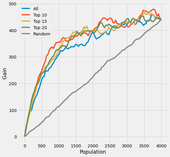
[30]:

df_preds = pd.DataFrame([y_preds.ravel(),
                         y_preds_t10.ravel(),
                         y_preds_t15.ravel(),
                         y_preds_t20.ravel(),
                         treatments,
                         df_test[y_name].ravel()],
                        index=['All', 'Top 10', 'Top 15', 'Top 20', 'is_treated', y_name]).T

plot_gain(df_preds, outcome_col=y_name, treatment_col='is_treated')

../_images/examples_feature_selection_42_0.png

[31]:

auuc_score(df_preds, outcome_col=y_name, treatment_col='is_treated')

[31]:

All       0.773405
Top 10    0.841204
Top 15    0.816100
Top 20    0.816252
Random    0.506801
dtype: float64

以R学习器为基础并输入随机森林回归器

[32]:

r_rf_learner = BaseRRegressor(
    RandomForestRegressor(
        n_estimators = 100,
        max_depth = 8,
        min_samples_leaf = 100
    ),
control_name='control')

[33]:

# using all features
features = X_names
r_rf_learner.fit(X = df_train[features].values,
                 treatment = df_train['treatment_group_key'].values,
                 y = df_train[y_name].values)
y_preds = r_rf_learner.predict(df_test[features].values)

INFO:causalml:Generating propensity score
INFO:causalml:Calibrating propensity scores.
INFO:causalml:generating out-of-fold CV outcome estimates
INFO:causalml:training the treatment effect model for treatment1 with R-loss

[34]:

# using top 10 features
features = top_10_features
r_rf_learner.fit(X = df_train[features].values,
                 treatment = df_train['treatment_group_key'].values,
                 y = df_train[y_name].values)
y_preds_t10 = r_rf_learner.predict(df_test[features].values)

INFO:causalml:Generating propensity score
INFO:causalml:Calibrating propensity scores.
INFO:causalml:generating out-of-fold CV outcome estimates
INFO:causalml:training the treatment effect model for treatment1 with R-loss

[35]:

# using top 15 features
features = top_15_features
r_rf_learner.fit(X = df_train[features].values,
                 treatment = df_train['treatment_group_key'].values,
                 y = df_train[y_name].values)
y_preds_t15 = r_rf_learner.predict(df_test[features].values)

INFO:causalml:Generating propensity score
INFO:causalml:Calibrating propensity scores.
INFO:causalml:generating out-of-fold CV outcome estimates
INFO:causalml:training the treatment effect model for treatment1 with R-loss

[36]:

# using top 20 features
features = top_20_features
r_rf_learner.fit(X = df_train[features].values,
                 treatment = df_train['treatment_group_key'].values,
                 y = df_train[y_name].values)
y_preds_t20 = r_rf_learner.predict(df_test[features].values)

INFO:causalml:Generating propensity score
INFO:causalml:Calibrating propensity scores.
INFO:causalml:generating out-of-fold CV outcome estimates
INFO:causalml:training the treatment effect model for treatment1 with R-loss

打印R学习器的结果

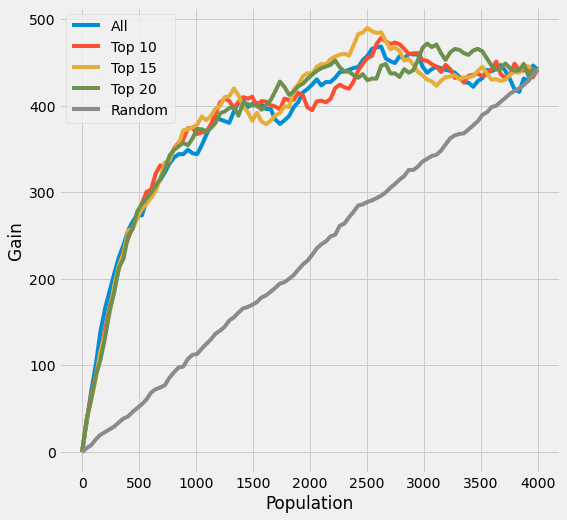
[37]:

df_preds = pd.DataFrame([y_preds.ravel(),
                         y_preds_t10.ravel(),
                         y_preds_t15.ravel(),
                         y_preds_t20.ravel(),
                         treatments,
                         df_test[y_name].ravel()],
                        index=['All', 'Top 10', 'Top 15', 'Top 20', 'is_treated', y_name]).T

plot_gain(df_preds, outcome_col=y_name, treatment_col='is_treated')

../_images/examples_feature_selection_51_0.png

[38]:

# print out AUUC score
auuc_score(df_preds, outcome_col=y_name, treatment_col='is_treated')

[38]:

All       0.859891
Top 10    0.865159
Top 15    0.872650
Top 20    0.870669
Random    0.506801
dtype: float64

（在这个R Learner案例中，AUUC的增强相对较小）

以S Learner为基础并输入随机森林回归器

[39]:

slearner_rf = BaseSRegressor(
    RandomForestRegressor(
        n_estimators = 100,
        max_depth = 8,
        min_samples_leaf = 100
    ),
    control_name='control')

[40]:

# using all features
features = X_names
slearner_rf.fit(X = df_train[features].values,
                treatment = df_train['treatment_group_key'].values,
                y = df_train[y_name].values)
y_preds = slearner_rf.predict(df_test[features].values)

[41]:

# using top 10 features
features = top_10_features
slearner_rf.fit(X = df_train[features].values,
                treatment = df_train['treatment_group_key'].values,
                y = df_train[y_name].values)
y_preds_t10 = slearner_rf.predict(df_test[features].values)

[42]:

# using top 15 features
features = top_15_features
slearner_rf.fit(X = df_train[features].values,
                treatment = df_train['treatment_group_key'].values,
                y = df_train[y_name].values)
y_preds_t15 = slearner_rf.predict(df_test[features].values)

[43]:

# using top 20 features
features = top_20_features
slearner_rf.fit(X = df_train[features].values,
                treatment = df_train['treatment_group_key'].values,
                y = df_train[y_name].values)
y_preds_t20 = slearner_rf.predict(df_test[features].values)

打印S Learner的结果

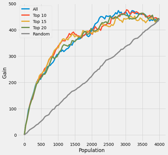
[44]:

df_preds = pd.DataFrame([y_preds.ravel(),
                         y_preds_t10.ravel(),
                         y_preds_t15.ravel(),
                         y_preds_t20.ravel(),
                         treatments,
                         df_test[y_name].ravel()],
                        index=['All', 'Top 10', 'Top 15', 'Top 20', 'is_treated', y_name]).T

plot_gain(df_preds, outcome_col=y_name, treatment_col='is_treated')

../_images/examples_feature_selection_61_0.png

[45]:

# print out AUUC score
auuc_score(df_preds, outcome_col=y_name, treatment_col='is_treated')

[45]:

All       0.824483
Top 10    0.832872
Top 15    0.817835
Top 20    0.816149
Random    0.506801
dtype: float64

在本笔记本中，我们展示了我们的Filter方法函数如何能够选择重要特征并提升AUUC性能（尽管结果可能因不同的数据集、模型和超参数而异）。

[ ]: