


NBA犯规分析与项目反应理论#
import os

import arviz as az
import matplotlib.pyplot as plt
import numpy as np
import pandas as pd
import pymc as pm

%matplotlib inline
print(f"Running on PyMC v{pm.__version__}")
Running on PyMC v4.0.0b6
RANDOM_SEED = 8927
rng = np.random.default_rng(RANDOM_SEED)
az.style.use("arviz-darkgrid")
介绍#
本教程展示了贝叶斯项目反应理论 [福克斯, 2010] 在NBA篮球犯规数据中的应用,使用PyMC。基于Austin Rochford的博客文章 NBA Foul Calls and Bayesian Item Response Theory。
动机#
我们的场景是,我们观察到一个二元结果(是否被判犯规),这个结果来自于两个具有不同角色(被指控犯规的球员和在比赛中处于不利地位的球员)的代理之间的互动(篮球比赛)。此外,每个犯规或处于不利地位的代理都是个体,可能会被多次观察到(例如,勒布朗·詹姆斯在多次比赛中被观察到犯规)。那么,可能不仅仅是代理的角色,单个球员的能力也会对观察到的结果产生影响。因此,我们希望估计每个个体(潜在)能力对观察到的结果的贡献,无论是作为犯规者还是处于不利地位的代理。这将使我们能够,例如,从更有效到更不有效对球员进行排名,量化这种排名的不确定性,并发现犯规判罚中涉及的额外层次结构。这些都是非常有用的信息!
那么,我们如何研究这种常见且复杂的多智能体交互场景,其中存在超过一千个个体之间的层次结构呢?
尽管场景的复杂性令人难以置信,贝叶斯项目反应理论结合现代强大的统计软件,提供了相当优雅且有效的建模选项。其中一种选项采用了称为广义线性模型的Rasch 模型,我们现在将更详细地讨论它。
Rasch 模型#
我们从官方的NBA Last Two Minutes Reports获取了2015年至2021年间的比赛数据。在这个数据集中,每一行k是一次涉及两名球员(犯规者和被侵犯者)的犯规事件,无论是否被裁判判罚。因此,我们将裁判在比赛k中判罚犯规的概率p_k建模为涉及球员的函数。因此,我们为每个球员定义了两个潜在变量,即:
theta: 估计球员在处于不利情况下被判犯规的能力,以及b: 估计球员在犯规时未被判罚的能力。
请注意,这些玩家的参数越高,对玩家所在的团队越有利。然后,通过假设p_k的对数几率等于参与比赛k的相应玩家的theta-b,使用标准的Rasch模型来估计这两个参数。此外,我们在所有theta和所有b上放置层次超先验,以解释玩家之间的共享能力和不同玩家之间观察数量的大量差异。
讨论#
我们的分析给出了每个玩家潜在技能theta和b的后验分布估计。我们通过三种方式分析这一结果。
我们首先展示共享超先验的作用,通过展示如何将观察较少的玩家的 posteriors 拉向联盟平均值。
其次,我们根据后验的均值对其进行排序,以查看最佳和最差的承诺和处于劣势的球员,并观察到在不同数据上估计的同一模型中,仍有几位球员排名在前10位,这与Austin Rochford博客文章中的结果一致。
第三,我们展示了如何发现按位置对支付者进行分组很可能会成为我们模型中引入的一个有信息量的额外层次结构,并将此作为对感兴趣的读者的练习。让我们最后提到,这种轻松地向模型中添加有信息的层次结构的机会是使贝叶斯建模在量化不确定性方面非常灵活和强大的特性之一,特别是在引入(或发现)特定问题的知识至关重要的场景中。
本笔记本中的分析分为四个主要步骤:
数据收集和处理。
Rasch 模型的定义和实例化。
后验采样和收敛性检查。
后验结果的分析。
数据收集与处理#
我们首先从原始数据集中导入数据,该数据集可以在此URL找到。每一行对应于NBA赛季2015-16至2020-21之间的比赛。我们只导入了五列,即
committing: 在游戏中提交操作的玩家名称。disadvantaged: 游戏中处于劣势的玩家的名称。decision: 比赛的审查决定,可以取四个值,即:CNC: 正确非调用,INC: 错误非调用,IC: 错误调用,CC: 正确调用.
committing_position: 提交玩家的位置,可以取值G: 后卫,F: 前锋,C: 中锋,G-F,F-G,F-C,C-F.
disadvantaged_position: 劣势玩家的位置,可能的值如上所述。
我们注意到,我们已经从原始数据集中移除了参与玩家少于两人的比赛(例如旅行呼叫或计时违规)。此外,原始数据集不包含玩家位置的信息,这是我们自己添加的。
try:
    df_orig = pd.read_csv(os.path.join("..", "data", "item_response_nba.csv"), index_col=0)
except FileNotFoundError:
    df_orig = pd.read_csv(pm.get_data("item_response_nba.csv"), index_col=0)
df_orig.head()
| committing | disadvantaged | decision | committing_position | disadvantaged_position | |
|---|---|---|---|---|---|
| play_id | |||||
| 1 | Avery Bradley | Stephen Curry | CNC | G | G |
| 3 | Isaiah Thomas | Andre Iguodala | CNC | G | G-F |
| 4 | Jae Crowder | Harrison Barnes | INC | F | F |
| 6 | Draymond Green | Isaiah Thomas | CC | F | G |
| 7 | Avery Bradley | Stephen Curry | CC | G | G |
我们现在分三个步骤处理我们的数据:
我们通过从
df_orig中移除位置信息来创建一个数据框df,并且我们创建一个数据框df_position来收集所有具有相应位置的球员。(这个最后的数据框直到笔记本的最后才会被使用。)我们向
df添加了一列,称为foul_called,如果判罚了犯规,则该列赋值为1,否则赋值为0。我们为有承诺和处于不利地位的玩家分配ID,并使用此索引来识别每次观察到的比赛中各自的玩家。
最后,我们显示主数据框 df 的头部以及一些基本统计数据。
# 1. Construct df and df_position
df = df_orig[["committing", "disadvantaged", "decision"]]

df_position = pd.concat(
    [
        df_orig.groupby("committing").committing_position.first(),
        df_orig.groupby("disadvantaged").disadvantaged_position.first(),
    ]
).to_frame()
df_position = df_position[~df_position.index.duplicated(keep="first")]
df_position.index.name = "player"
df_position.columns = ["position"]


# 2. Create the binary foul_called variable
def foul_called(decision):
    """Correct and incorrect noncalls (CNC and INC) take value 0.
    Correct and incorrect calls (CC and IC) take value 1.
    """
    out = 0
    if (decision == "CC") | (decision == "IC"):
        out = 1
    return out


df = df.assign(foul_called=lambda df: df["decision"].apply(foul_called))

# 3 We index observed calls by committing and disadvantaged players
committing_observed, committing = pd.factorize(df.committing, sort=True)
disadvantaged_observed, disadvantaged = pd.factorize(df.disadvantaged, sort=True)
df.index.name = "play_id"

# Display of main dataframe with some statistics
print(f"Number of observed plays: {len(df)}")
print(f"Number of disadvantaged players: {len(disadvantaged)}")
print(f"Number of committing players: {len(committing)}")
print(f"Global probability of a foul being called: " f"{100*round(df.foul_called.mean(),3)}%\n\n")
df.head()
Number of observed plays: 46861
Number of disadvantaged players: 770
Number of committing players: 789
Global probability of a foul being called: 23.3%
| committing | disadvantaged | decision | foul_called | |
|---|---|---|---|---|
| play_id | ||||
| 1 | Avery Bradley | Stephen Curry | CNC | 0 |
| 3 | Isaiah Thomas | Andre Iguodala | CNC | 0 |
| 4 | Jae Crowder | Harrison Barnes | INC | 0 |
| 6 | Draymond Green | Isaiah Thomas | CC | 1 |
| 7 | Avery Bradley | Stephen Curry | CC | 1 |
项目反应模型#
模型定义#
我们表示为:
\(N_d\) 和 \(N_c\) 分别表示处于不利地位和实施行为的玩家数量,
\(K\) 游戏次数,
\(k\) 一场戏,
\(y_k\) 比赛中观察到的呼叫/非呼叫 \(k\),
\(p_k\) 比赛中犯规被判罚的概率 \(k\),
\(i(k)\) 游戏 \(k\) 中的劣势玩家,以及由
\(j(k)\) 在游戏 \(k\) 中的承诺玩家。
我们假设每个处于不利地位的玩家由潜在变量描述:
\(\theta_i\) 对于 \(i=1,2,...,N_d\),
每个提交的玩家由潜在变量描述:
\(b_j\) 对于 \(j=1,2,...,N_c\)。
然后我们将每个观测值 \(y_k\) 建模为具有概率 \(p_k\) 的独立伯努利试验的结果,其中
对于 \(k=1,2,...,K\),通过定义(通过非中心参数化)
带有先验/超先验
请注意,\(p_k\) 总是依赖于 \(\mu_\theta,\,\sigma_\theta\) 和 \(\sigma_b\)(“合并先验”),并且由于 \(\Delta_{\theta,i}\) 和 \(\Delta_{b,j}\)(“未合并先验”),还依赖于实际参与比赛的玩家。这意味着我们的模型具有部分合并的特点。此外,请注意,我们没有将 \(\theta\) 与 \(b\) 合并,因此假设这些技能即使对于同一玩家也是独立的。另外,请注意,我们将 \(b_{j}\) 的均值归一化为零。
最后,请注意我们是如何从数据出发,反向构建这个模型的。这是一种非常自然的构建模型的方法,使我们能够快速了解每个变量如何与其他变量连接及其直觉。同时,在下面的模型实例化中,构建过程是相反的,即从先验开始,逐步上升到观测值。
PyMC 实现#
我们现在在 PyMC 中实现上述模型。请注意,为了轻松跟踪玩家(因为我们有数百名玩家既是施害者也是受害者),我们使用了 coords 参数用于 pymc.Model。(有关此功能的教程,请参阅笔记本 使用数据容器 或 这篇博客文章。)我们选择先验与 Austin Rochford 的文章 中的相同,以确保比较的一致性。
coords = {"disadvantaged": disadvantaged, "committing": committing}

with pm.Model(coords=coords) as model:
    # Data
    foul_called_observed = pm.Data("foul_called_observed", df.foul_called, mutable=False)

    # Hyperpriors
    mu_theta = pm.Normal("mu_theta", 0.0, 100.0)
    sigma_theta = pm.HalfCauchy("sigma_theta", 2.5)
    sigma_b = pm.HalfCauchy("sigma_b", 2.5)

    # Priors
    Delta_theta = pm.Normal("Delta_theta", 0.0, 1.0, dims="disadvantaged")
    Delta_b = pm.Normal("Delta_b", 0.0, 1.0, dims="committing")

    # Deterministic
    theta = pm.Deterministic("theta", Delta_theta * sigma_theta + mu_theta, dims="disadvantaged")
    b = pm.Deterministic("b", Delta_b * sigma_b, dims="committing")
    eta = pm.Deterministic("eta", theta[disadvantaged_observed] - b[committing_observed])

    # Likelihood
    y = pm.Bernoulli("y", logit_p=eta, observed=foul_called_observed)
我们现在绘制我们的模型,以展示在变量 theta 和 b 上的层次结构(以及非中心参数化)。
pm.model_to_graphviz(model)

采样与收敛#
我们现在从Rasch模型中进行采样。
with model:
    trace = pm.sample(1000, tune=1500, random_seed=RANDOM_SEED)
Auto-assigning NUTS sampler...
Initializing NUTS using jitter+adapt_diag...
Multiprocess sampling (4 chains in 4 jobs)
NUTS: [mu_theta, sigma_theta, sigma_b, Delta_theta, Delta_b]
Sampling 4 chains for 1_500 tune and 1_000 draw iterations (6_000 + 4_000 draws total) took 431 seconds.
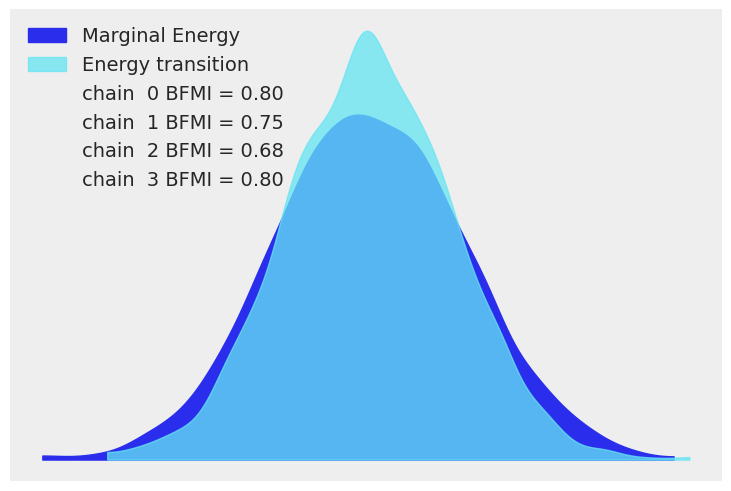
我们在下面绘制了所得轨迹的能量差。此外,我们假设我们的采样器已经收敛,因为它通过了所有自动的PyMC收敛检查。
az.plot_energy(trace);
后验分析#
部分池化的可视化#
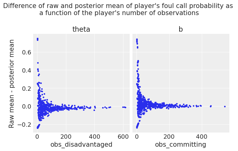
我们的第一个检查是绘制
y: 每个处于不利地位和有行为的玩家的原始平均概率(来自数据)与后验平均概率之间的差异
x: 作为每个处于不利地位和有不良行为的玩家观察数量的函数。
这些图表显示,正如预期的那样,我们模型的层次结构倾向于将观察量较少的玩家的估计后验值向全局均值靠拢。
# Global posterior means of μ_theta and μ_b
mu_theta_mean, mu_b_mean = trace.posterior["mu_theta"].mean(), 0
# Raw mean from data of each disadvantaged player
disadvantaged_raw_mean = df.groupby("disadvantaged")["foul_called"].mean()
# Raw mean from data of each committing player
committing_raw_mean = df.groupby("committing")["foul_called"].mean()
# Posterior mean of each disadvantaged player
disadvantaged_posterior_mean = (
    1 / (1 + np.exp(-trace.posterior["theta"].mean(dim=["chain", "draw"]))).to_pandas()
)
# Posterior mean of each committing player
committing_posterior_mean = (
    1
    / (1 + np.exp(-(mu_theta_mean - trace.posterior["b"].mean(dim=["chain", "draw"])))).to_pandas()
)


# Compute difference of raw and posterior mean for each
# disadvantaged and committing player
def diff(a, b):
    return a - b


df_disadvantaged = pd.DataFrame(
    disadvantaged_raw_mean.combine(disadvantaged_posterior_mean, diff),
    columns=["Raw - posterior mean"],
)
df_committing = pd.DataFrame(
    committing_raw_mean.combine(committing_posterior_mean, diff), columns=["Raw - posterior mean"]
)
# Add the number of observations for each disadvantaged and committing player
df_disadvantaged = df_disadvantaged.assign(obs_disadvantaged=df["disadvantaged"].value_counts())
df_committing = df_committing.assign(obs_committing=df["committing"].value_counts())

# Plot the difference between raw and posterior means as a function of
# the number of observations
fig, (ax1, ax2) = plt.subplots(1, 2, sharey=True)
fig.suptitle(
    "Difference of raw and posterior mean of player's foul call probability as "
    "\na function of the player's number of observations\n",
    fontsize=15,
)
ax1.scatter(data=df_disadvantaged, x="obs_disadvantaged", y="Raw - posterior mean", s=7, marker="o")
ax1.set_title("theta")
ax1.set_ylabel("Raw mean - posterior mean")
ax1.set_xlabel("obs_disadvantaged")
ax2.scatter(data=df_committing, x="obs_committing", y="Raw - posterior mean", s=7)
ax2.set_title("b")
ax2.set_xlabel("obs_committing")
plt.show()
顶部和底部提交和处于不利地位的玩家#
正如我们成功估计了劣势玩家(theta)和进攻玩家(b)的技能,我们最终可以检查在我们的模型中哪些玩家表现更好或更差。
因此,我们现在使用森林图绘制我们的后验分布。我们分别绘制了根据潜在技能theta和b排名的前10名和后10名玩家。
def order_posterior(inferencedata, var, bottom_bool):
    xarray_ = inferencedata.posterior[var].mean(dim=["chain", "draw"])
    return xarray_.sortby(xarray_, ascending=bottom_bool)


top_theta, bottom_theta = (
    order_posterior(trace, "theta", False),
    order_posterior(trace, "theta", True),
)
top_b, bottom_b = (order_posterior(trace, "b", False), order_posterior(trace, "b", True))

amount = 10  # How many top players we want to display in each cathegory

fig = plt.figure(figsize=(17, 14))
fig.suptitle(
    "\nPosterior estimates for top and bottom disadvantaged (theta) and "
    "committing (b) players \n(94% HDI)\n",
    fontsize=25,
)
theta_top_ax = fig.add_subplot(221)
b_top_ax = fig.add_subplot(222)
theta_bottom_ax = fig.add_subplot(223, sharex=theta_top_ax)
b_bottom_ax = fig.add_subplot(224, sharex=b_top_ax)

# theta: plot top
az.plot_forest(
    trace,
    var_names=["theta"],
    combined=True,
    coords={"disadvantaged": top_theta["disadvantaged"][:amount]},
    ax=theta_top_ax,
    labeller=az.labels.NoVarLabeller(),
)
theta_top_ax.set_title(f"theta: top {amount}")
theta_top_ax.set_xlabel("theta\n")
theta_top_ax.set_xlim(xmin=-2.5, xmax=0.1)
theta_top_ax.vlines(mu_theta_mean, -1, amount, "k", "--", label=("League average"))
theta_top_ax.legend(loc=2)


# theta: plot bottom
az.plot_forest(
    trace,
    var_names=["theta"],
    colors="blue",
    combined=True,
    coords={"disadvantaged": bottom_theta["disadvantaged"][:amount]},
    ax=theta_bottom_ax,
    labeller=az.labels.NoVarLabeller(),
)
theta_bottom_ax.set_title(f"theta: bottom {amount}")
theta_bottom_ax.set_xlabel("theta")
theta_bottom_ax.vlines(mu_theta_mean, -1, amount, "k", "--", label=("League average"))
theta_bottom_ax.legend(loc=2)

# b: plot top
az.plot_forest(
    trace,
    var_names=["b"],
    colors="blue",
    combined=True,
    coords={"committing": top_b["committing"][:amount]},
    ax=b_top_ax,
    labeller=az.labels.NoVarLabeller(),
)
b_top_ax.set_title(f"b: top {amount}")
b_top_ax.set_xlabel("b\n")
b_top_ax.set_xlim(xmin=-1.5, xmax=1.5)
b_top_ax.vlines(0, -1, amount, "k", "--", label="League average")
b_top_ax.legend(loc=2)

# b: plot bottom
az.plot_forest(
    trace,
    var_names=["b"],
    colors="blue",
    combined=True,
    coords={"committing": bottom_b["committing"][:amount]},
    ax=b_bottom_ax,
    labeller=az.labels.NoVarLabeller(),
)
b_bottom_ax.set_title(f"b: bottom {amount}")
b_bottom_ax.set_xlabel("b")
b_bottom_ax.vlines(0, -1, amount, "k", "--", label="League average")
b_bottom_ax.legend(loc=2)
plt.show();
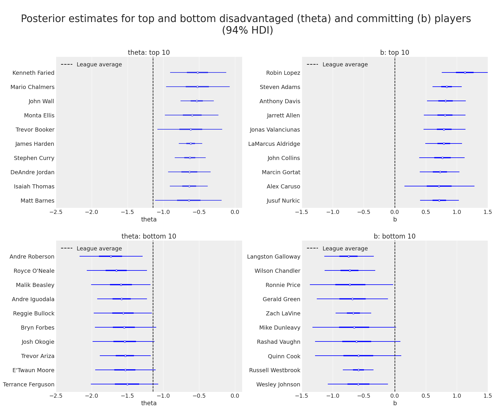
通过访问Austin Rochford的文章并查看那里的Rasch模型的类似表格(使用2016-17赛季的数据),读者可以看到,在我们的更大数据集(涵盖2015-16至2020-21赛季)中,许多顶级球员在两项技能中仍然位居前十。
发现额外的层次结构#
一个自然的问题是,作为处于不利地位的玩家(即具有高theta的玩家)是否也可能是擅长作为违规玩家(即具有高b的玩家),反之亦然。因此,接下来的两个图显示了相对于b(分别theta)的顶级玩家的theta(分别b)得分。
amount = 20  # How many top players we want to display
top_theta_players = top_theta["disadvantaged"][:amount].values
top_b_players = top_b["committing"][:amount].values

top_theta_in_committing = set(committing).intersection(set(top_theta_players))
top_b_in_disadvantaged = set(disadvantaged).intersection(set(top_b_players))
if (len(top_theta_in_committing) < amount) | (len(top_b_in_disadvantaged) < amount):
    print(
        f"Some players in the top {amount} for theta (or b) do not have observations for b (or theta).\n",
        "Plot not shown",
    )
else:
    fig = plt.figure(figsize=(17, 14))
    fig.suptitle(
        "\nScores as committing (b) for best disadvantaged (theta) players"
        " and vice versa"
        "\n(94% HDI)\n",
        fontsize=25,
    )
    b_top_theta = fig.add_subplot(121)
    theta_top_b = fig.add_subplot(122)

    az.plot_forest(
        trace,
        var_names=["b"],
        colors="blue",
        combined=True,
        coords={"committing": top_theta_players},
        figsize=(7, 7),
        ax=b_top_theta,
        labeller=az.labels.NoVarLabeller(),
    )
    b_top_theta.set_title(f"\nb score for top {amount} in theta\n (94% HDI)\n\n", fontsize=17)
    b_top_theta.set_xlabel("b")
    b_top_theta.vlines(mu_b_mean, -1, amount, color="k", ls="--", label="League average")
    b_top_theta.legend(loc="upper right", bbox_to_anchor=(0.46, 1.05))

    az.plot_forest(
        trace,
        var_names=["theta"],
        colors="blue",
        combined=True,
        coords={"disadvantaged": top_b_players},
        figsize=(7, 7),
        ax=theta_top_b,
        labeller=az.labels.NoVarLabeller(),
    )
    theta_top_b.set_title(f"\ntheta score for top {amount} in b\n (94% HDI)\n\n", fontsize=17)
    theta_top_b.set_xlabel("theta")
    theta_top_b.vlines(mu_theta_mean, -1, amount, color="k", ls="--", label="League average")
    theta_top_b.legend(loc="upper right", bbox_to_anchor=(0.46, 1.05));
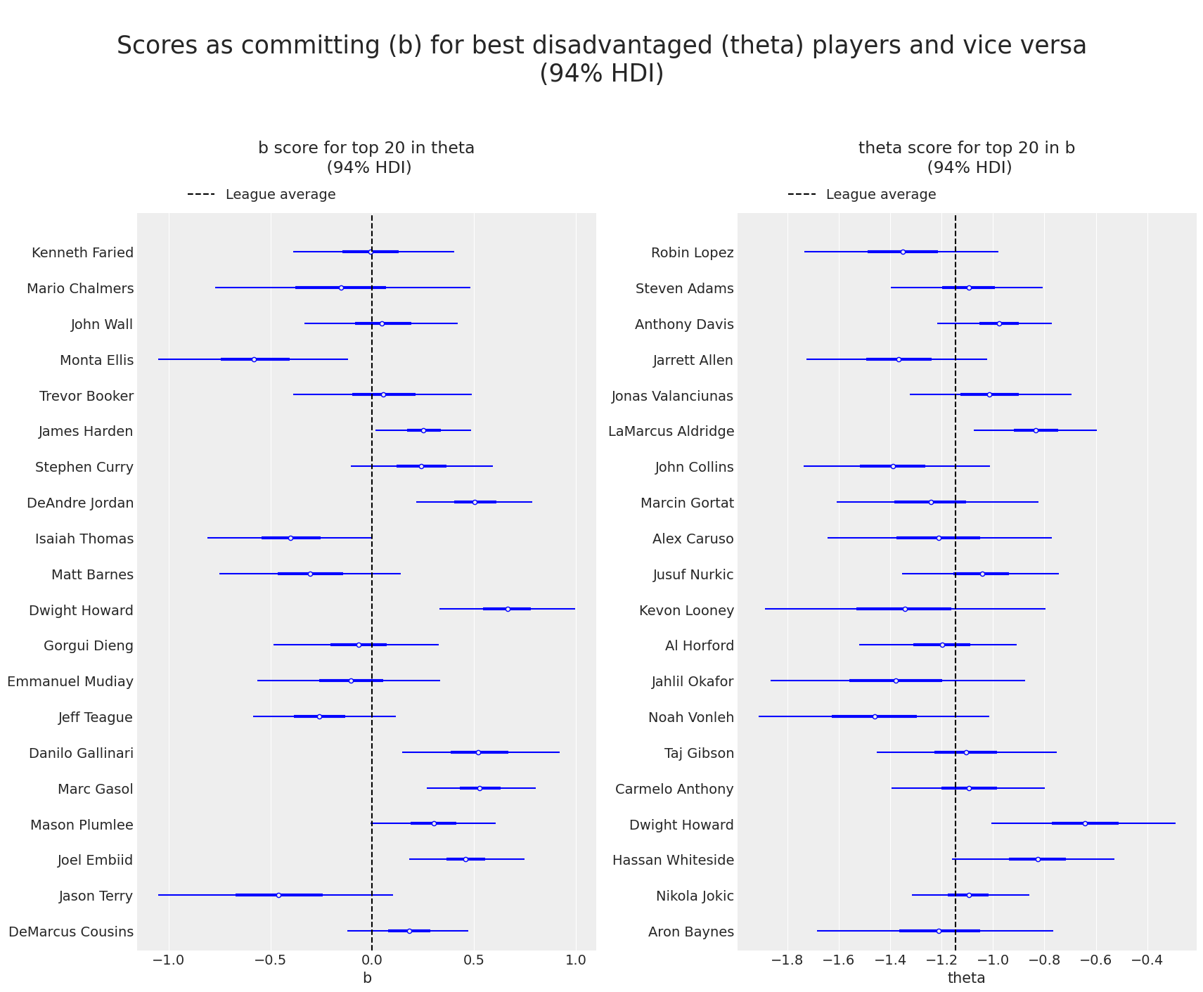
这些图表表明,在theta中得分高与在b中得分高低没有关联。此外,凭借对NBA篮球的一点了解,人们可以直观地注意到,在b中得分较高的球员更可能是中锋或前锋,而不是后卫或控球后卫。
鉴于最后的观察,我们决定绘制一个直方图,显示在顶级不利(theta)和犯规(b)球员中不同位置的出现频率。有趣的是,我们发现以下情况:最佳不利球员中最大比例的是后卫,而最佳犯规球员中最大比例的是中锋(同时后卫的比例非常小)。
amount = 50  # How many top players we want to display
top_theta_players = top_theta["disadvantaged"][:amount].values
top_b_players = top_b["committing"][:amount].values

positions = ["C", "C-F", "F-C", "F", "G-F", "G"]

# Histogram of positions of top disadvantaged players
fig = plt.figure(figsize=(8, 6))
top_theta_position = fig.add_subplot(121)
df_position.loc[df_position.index.isin(top_theta_players)].position.value_counts().loc[
    positions
].plot.bar(ax=top_theta_position, color="orange", label="theta")
top_theta_position.set_title(f"Positions of top {amount} disadvantaged (theta)\n", fontsize=12)
top_theta_position.legend(loc="upper left")

# Histogram of positions of top committing players
top_b_position = fig.add_subplot(122, sharey=top_theta_position)
df_position.loc[df_position.index.isin(top_b_players)].position.value_counts().loc[
    positions
].plot.bar(ax=top_b_position, label="b")
top_b_position.set_title(f"Positions of top {amount} committing (b)\n", fontsize=12)
top_b_position.legend(loc="upper right");
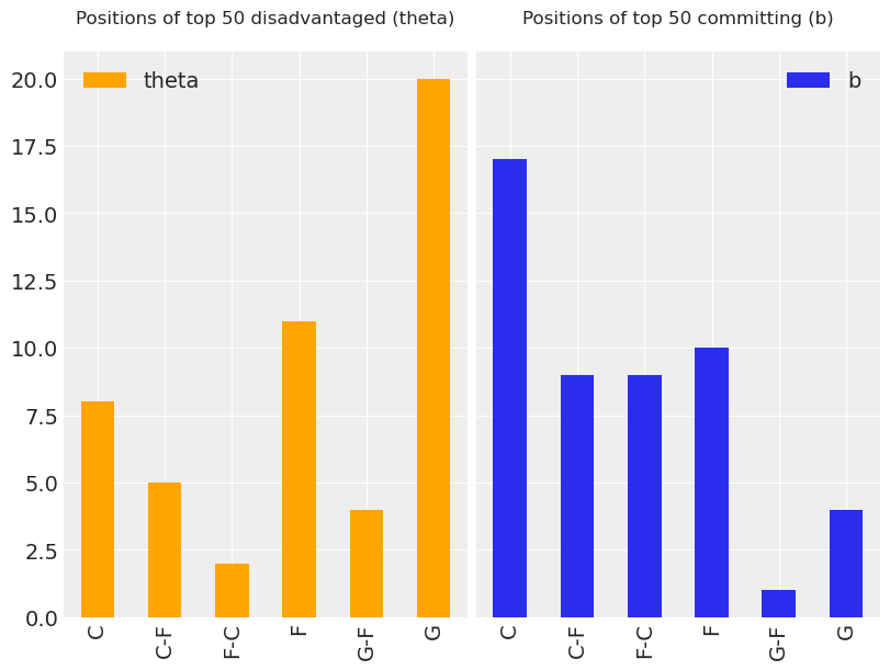
上面的直方图表明,在我们的模型中添加一个层次结构可能是合适的。即,根据各自的位置将处于不利地位和有不良行为的球员分组,以考虑位置在评估潜在技能theta和b中的作用。这可以通过在我们的Rasch模型中为每个按位置分组的球员施加均值和方差超先验来实现,这留给读者作为练习。为此,请注意数据框df_orig正是为了添加这种层次结构而设置的。祝你玩得开心!
衷心感谢 Eric Ma 提供了许多有用的评论,这些评论改进了这个笔记本。
参考资料#
让-保罗·福克斯。贝叶斯项目反应建模:理论与应用。斯普林格,2010年。
水印#
%load_ext watermark
%watermark -n -u -v -iv -w -p pytensor,aeppl,xarray
Last updated: Sat Apr 23 2022

Python implementation: CPython
Python version       : 3.9.12
IPython version      : 8.2.0

pytensor: 2.6.2
aeppl : 0.0.28
xarray: 2022.3.0

matplotlib: 3.5.1
numpy     : 1.22.3
pymc      : 4.0.0b6
arviz     : 0.13.0.dev0
pandas    : 1.4.2

Watermark: 2.3.0