使用PyMC将强化学习模型拟合到行为数据

强化学习模型通常用于行为研究中，以模拟动物和人类在可以进行重复选择并随后获得某种形式的反馈（如奖励或惩罚）的情况下如何学习。

在本笔记本中，我们将考虑最简单的学习场景，其中只有两种可能的动作。当采取一个动作时，它总是紧随一个即时的奖励。最后，每个动作的结果与之前采取的动作无关。这种情况有时被称为多臂赌博机问题。

假设两个动作（例如，左按钮和右按钮）分别有40%和60%的时间与单位奖励相关联。在开始时，学习代理不知道哪个动作 \(a\) 更好，因此它们可能从假设两个动作的平均值都是50%开始。我们可以将这些值存储在一个表中，这个表通常被称为 \(Q\) 表：

\[\begin{split} Q = \begin{cases} .5, a = \text{left}\\ .5, a = \text{right} \end{cases} \end{split}\]

当选择一个动作并观察到奖励 \(r = \{0,1\}\) 时，该动作的估计值更新如下：

\[Q_{a} = Q_{a} + \alpha (r - Q_{a})\]

其中 \(\alpha \in [0, 1]\) 是一个学习参数，它影响在每次试验中动作值向观察到的奖励的偏移程度。最后，\(Q\) 表的值通过 softmax 变换转换为动作概率：

\[ P(a = \text{right}) = \frac{\exp(\beta Q_{\text{right}})}{\exp(\beta Q_{\text{right}}) + \exp(\beta Q_{\text{left}})}\]

其中参数 \(\beta \in (0, +\infty)\) 决定了代理选择的噪声水平。较大的值将对应于更确定的选择，而较小的值将对应于越来越随机的选择。

import arviz as az
import matplotlib.pyplot as plt
import numpy as np
import pymc as pm
import pytensor
import pytensor.tensor as pt
import scipy

from matplotlib.lines import Line2D

seed = sum(map(ord, "RL_PyMC"))
rng = np.random.default_rng(seed)
az.style.use("arviz-darkgrid")
%config InlineBackend.figure_format = "retina"

生成假数据

def generate_data(rng, alpha, beta, n=100, p_r=None):
    if p_r is None:
        p_r = [0.4, 0.6]
    actions = np.zeros(n, dtype="int")
    rewards = np.zeros(n, dtype="int")
    Qs = np.zeros((n, 2))

    # Initialize Q table
    Q = np.array([0.5, 0.5])
    for i in range(n):
        # Apply the Softmax transformation
        exp_Q = np.exp(beta * Q)
        prob_a = exp_Q / np.sum(exp_Q)

        # Simulate choice and reward
        a = rng.choice([0, 1], p=prob_a)
        r = rng.random() < p_r[a]

        # Update Q table
        Q[a] = Q[a] + alpha * (r - Q[a])

        # Store values
        actions[i] = a
        rewards[i] = r
        Qs[i] = Q.copy()

    return actions, rewards, Qs

true_alpha = 0.5
true_beta = 5
n = 150
actions, rewards, Qs = generate_data(rng, true_alpha, true_beta, n)

Show code cell source Hide code cell source

_, ax = plt.subplots(figsize=(12, 5))
x = np.arange(len(actions))

ax.plot(x, Qs[:, 0] - 0.5 + 0, c="C0", lw=3, alpha=0.3)
ax.plot(x, Qs[:, 1] - 0.5 + 1, c="C1", lw=3, alpha=0.3)

s = 7
lw = 2

cond = (actions == 0) & (rewards == 0)
ax.plot(x[cond], actions[cond], "o", ms=s, mfc="None", mec="C0", mew=lw)

cond = (actions == 0) & (rewards == 1)
ax.plot(x[cond], actions[cond], "o", ms=s, mfc="C0", mec="C0", mew=lw)

cond = (actions == 1) & (rewards == 0)
ax.plot(x[cond], actions[cond], "o", ms=s, mfc="None", mec="C1", mew=lw)

cond = (actions == 1) & (rewards == 1)
ax.plot(x[cond], actions[cond], "o", ms=s, mfc="C1", mec="C1", mew=lw)

ax.set_yticks([0, 1], ["left", "right"])
ax.set_ylim(-1, 2)
ax.set_ylabel("action")
ax.set_xlabel("trial")

reward_artist = Line2D([], [], c="k", ls="none", marker="o", ms=s, mew=lw, label="Reward")
no_reward_artist = Line2D(
    [], [], ls="none", marker="o", mfc="w", mec="k", ms=s, mew=lw, label="No reward"
)
Qvalue_artist = Line2D([], [], c="k", ls="-", lw=3, alpha=0.3, label="Qvalue (centered)")

ax.legend(handles=[no_reward_artist, Qvalue_artist, reward_artist], fontsize=12, loc=(1.01, 0.27));

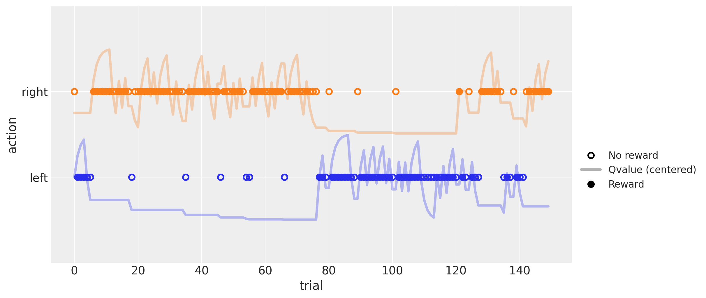
上图显示了150次试验的模拟运行，参数为\(\alpha = .5\)和\(\beta = 5\)，左侧（蓝色）和右侧（橙色）动作的常数奖励概率分别为\(.4\)和\(.6\)。

实心点和空心点分别表示跟随奖励和无奖励的动作。实线显示了围绕各自彩色点的每个动作的估计\(Q\)值（当各自的\(Q\)值高于\(.5\)时，线条在其点上方，否则在其下方）。可以看出，该值随着奖励（实心点）增加，随着无奖励（空心点）减少。

每次结果后行高的变化直接与\(\alpha\)参数相关。\(\beta\)参数的影响更难理解，但一种思考方式是，其值越高，代理就越会坚持执行估计值最高的动作，即使两者之间的差异非常小。相反，当这个值接近零时，代理将开始在两个动作之间随机选择，而不考虑它们的估计值。

通过最大似然估计学习参数

生成数据后，目标是现在“反转模型”以估计学习参数 \(\alpha\) 和 \(\beta\)。我首先通过最大似然估计（MLE）来实现这一点。这需要编写一个自定义函数，该函数计算给定潜在 \(\alpha\) 和 \(\beta\) 以及固定的观察到的动作和奖励的数据的可能性（实际上，该函数计算负对数似然，以避免下溢问题）。

我使用方便的 scipy.optimize.minimize 函数，快速获取使数据似然性最大化的 \(\alpha\) 和 \(\beta\) 值（实际上，是使负对数似然最小化）。

这在后来我编写计算 PyMC 中选择概率的 PyTensor 函数时也很有帮助。首先，底层逻辑是相同的，唯一改变的是语法。其次，它提供了一种方式，让我确信我没有搞错，我实际计算的就是我想要计算的内容。

def llik_td(x, *args):
    # Extract the arguments as they are passed by scipy.optimize.minimize
    alpha, beta = x
    actions, rewards = args

    # Initialize values
    Q = np.array([0.5, 0.5])
    logp_actions = np.zeros(len(actions))

    for t, (a, r) in enumerate(zip(actions, rewards)):
        # Apply the softmax transformation
        Q_ = Q * beta
        logp_action = Q_ - scipy.special.logsumexp(Q_)

        # Store the log probability of the observed action
        logp_actions[t] = logp_action[a]

        # Update the Q values for the next trial
        Q[a] = Q[a] + alpha * (r - Q[a])

    # Return the negative log likelihood of all observed actions
    return -np.sum(logp_actions[1:])

函数 llik_td 与 generate_data 非常相似，不同之处在于它不是在每次试验中模拟一个动作和奖励，而是存储观察到的动作的对数概率。

函数 scipy.special.logsumexp 用于以一种更数值稳定的方式计算项 \(\log(\exp(\beta Q_{\text{right}}) + \exp(\beta Q_{\text{left}}))\)。

最终，函数返回所有对数概率的负和，这相当于在其原始尺度上乘以概率。

（第一个动作被忽略，只是为了让输出与后面的 PyTensor 函数相比较。它实际上不会改变任何估计，因为初始概率是固定的，不依赖于 \(\alpha\) 或 \(\beta\) 参数。）

llik_td([true_alpha, true_beta], *(actions, rewards))

47.418936097207016

上面，我计算了给定真实\(\alpha\)和\(\beta\)参数的数据的负对数似然。

下面，我让scipy找到两个参数的最大似然估计值：

x0 = [true_alpha, true_beta]
result = scipy.optimize.minimize(llik_td, x0, args=(actions, rewards), method="BFGS")
print(result)
print("")
print(f"MLE: alpha = {result.x[0]:.2f} (true value = {true_alpha})")
print(f"MLE: beta = {result.x[1]:.2f} (true value = {true_beta})")

      fun: 47.050814541102895
 hess_inv: array([[ 0.00733307, -0.02421781],
       [-0.02421781,  0.86969299]])
      jac: array([0., 0.])
  message: 'Optimization terminated successfully.'
     nfev: 30
      nit: 7
     njev: 10
   status: 0
  success: True
        x: array([0.50473117, 5.7073849 ])

MLE: alpha = 0.50 (true value = 0.5)
MLE: beta = 5.71 (true value = 5)

估计的最大似然估计值与真实值相对接近。然而，这种方法并没有给出这些参数值周围可能的不确定性的任何概念。为了得到这一点，我将转向PyMC进行贝叶斯后验估计。

但在那之前，我将对对数似然函数实现一个简单的向量化优化，这将更类似于 PyTensor 的对应部分。这样做的目的是为了加快未来的贝叶斯推理引擎的速度。

def llik_td_vectorized(x, *args):
    # Extract the arguments as they are passed by scipy.optimize.minimize
    alpha, beta = x
    actions, rewards = args

    # Create a list with the Q values of each trial
    Qs = np.ones((n, 2), dtype="float64")
    Qs[0] = 0.5
    for t, (a, r) in enumerate(
        zip(actions[:-1], rewards[:-1])
    ):  # The last Q values were never used, so there is no need to compute them
        Qs[t + 1, a] = Qs[t, a] + alpha * (r - Qs[t, a])
        Qs[t + 1, 1 - a] = Qs[t, 1 - a]

    # Apply the softmax transformation in a vectorized way
    Qs_ = Qs * beta
    logp_actions = Qs_ - scipy.special.logsumexp(Qs_, axis=1)[:, None]

    # Return the logp_actions for the observed actions
    logp_actions = logp_actions[np.arange(len(actions)), actions]
    return -np.sum(logp_actions[1:])

llik_td_vectorized([true_alpha, true_beta], *(actions, rewards))

47.418936097207016

%timeit llik_td([true_alpha, true_beta], *(actions, rewards))

7.13 ms ± 832 µs per loop (mean ± std. dev. of 7 runs, 100 loops each)

%timeit llik_td_vectorized([true_alpha, true_beta], *(actions, rewards))

653 µs ± 119 µs per loop (mean ± std. dev. of 7 runs, 1,000 loops each)

矢量化函数给出了相同的结果，但运行速度几乎快了一个数量级。

当作为PyTensor函数实现时，向量化版本和标准版本之间的差异并没有这么大。尽管如此，它的运行速度仍然是标准版本的两倍，这意味着模型的采样速度也是标准版本的两倍！

通过PyMC估计学习参数

最具挑战性的部分是创建一个 PyTensor 函数/循环，以便在使用 PyMC 采样参数时估计 Q 值。

def update_Q(action, reward, Qs, alpha):
    """
    This function updates the Q table according to the RL update rule.
    It will be called by pytensor.scan to do so recursevely, given the observed data and the alpha parameter
    This could have been replaced be the following lamba expression in the pytensor.scan fn argument:
        fn=lamba action, reward, Qs, alpha: pt.set_subtensor(Qs[action], Qs[action] + alpha * (reward - Qs[action]))
    """

    Qs = pt.set_subtensor(Qs[action], Qs[action] + alpha * (reward - Qs[action]))
    return Qs

# Transform the variables into appropriate PyTensor objects
rewards_ = pt.as_tensor_variable(rewards, dtype="int32")
actions_ = pt.as_tensor_variable(actions, dtype="int32")

alpha = pt.scalar("alpha")
beta = pt.scalar("beta")

# Initialize the Q table
Qs = 0.5 * pt.ones((2,), dtype="float64")

# Compute the Q values for each trial
Qs, _ = pytensor.scan(
    fn=update_Q, sequences=[actions_, rewards_], outputs_info=[Qs], non_sequences=[alpha]
)

# Apply the softmax transformation
Qs = Qs * beta
logp_actions = Qs - pt.logsumexp(Qs, axis=1, keepdims=True)

# Calculate the negative log likelihod of the observed actions
logp_actions = logp_actions[pt.arange(actions_.shape[0] - 1), actions_[1:]]
neg_loglike = -pt.sum(logp_actions)

让我们将其封装在一个函数中，以测试它是否按预期工作。

pytensor_llik_td = pytensor.function(
    inputs=[alpha, beta], outputs=neg_loglike, on_unused_input="ignore"
)
result = pytensor_llik_td(true_alpha, true_beta)
float(result)

47.418936097206995

得到了相同的结果，因此我们可以确信 PyTensor 循环按预期工作。我们现在准备实现 PyMC 模型。

def pytensor_llik_td(alpha, beta, actions, rewards):
    rewards = pt.as_tensor_variable(rewards, dtype="int32")
    actions = pt.as_tensor_variable(actions, dtype="int32")

    # Compute the Qs values
    Qs = 0.5 * pt.ones((2,), dtype="float64")
    Qs, updates = pytensor.scan(
        fn=update_Q, sequences=[actions, rewards], outputs_info=[Qs], non_sequences=[alpha]
    )

    # Apply the sotfmax transformation
    Qs = Qs[:-1] * beta
    logp_actions = Qs - pt.logsumexp(Qs, axis=1, keepdims=True)

    # Calculate the log likelihood of the observed actions
    logp_actions = logp_actions[pt.arange(actions.shape[0] - 1), actions[1:]]
    return pt.sum(logp_actions)  # PyMC expects the standard log-likelihood

with pm.Model() as m:
    alpha = pm.Beta(name="alpha", alpha=1, beta=1)
    beta = pm.HalfNormal(name="beta", sigma=10)

    like = pm.Potential(name="like", var=pytensor_llik_td(alpha, beta, actions, rewards))

    tr = pm.sample(random_seed=rng)

Auto-assigning NUTS sampler...
Initializing NUTS using jitter+adapt_diag...
Multiprocess sampling (4 chains in 4 jobs)
NUTS: [alpha, beta]

100.00% [8000/8000 00:25<00:00 Sampling 4 chains, 0 divergences]

Sampling 4 chains for 1_000 tune and 1_000 draw iterations (4_000 + 4_000 draws total) took 48 seconds.

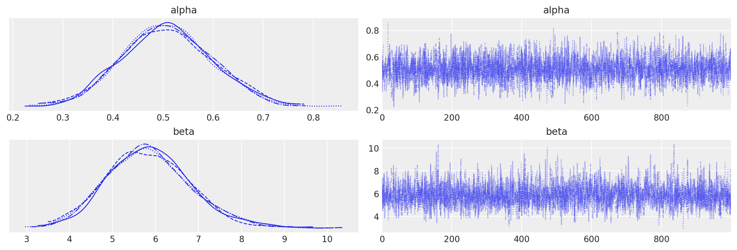
az.plot_trace(data=tr);

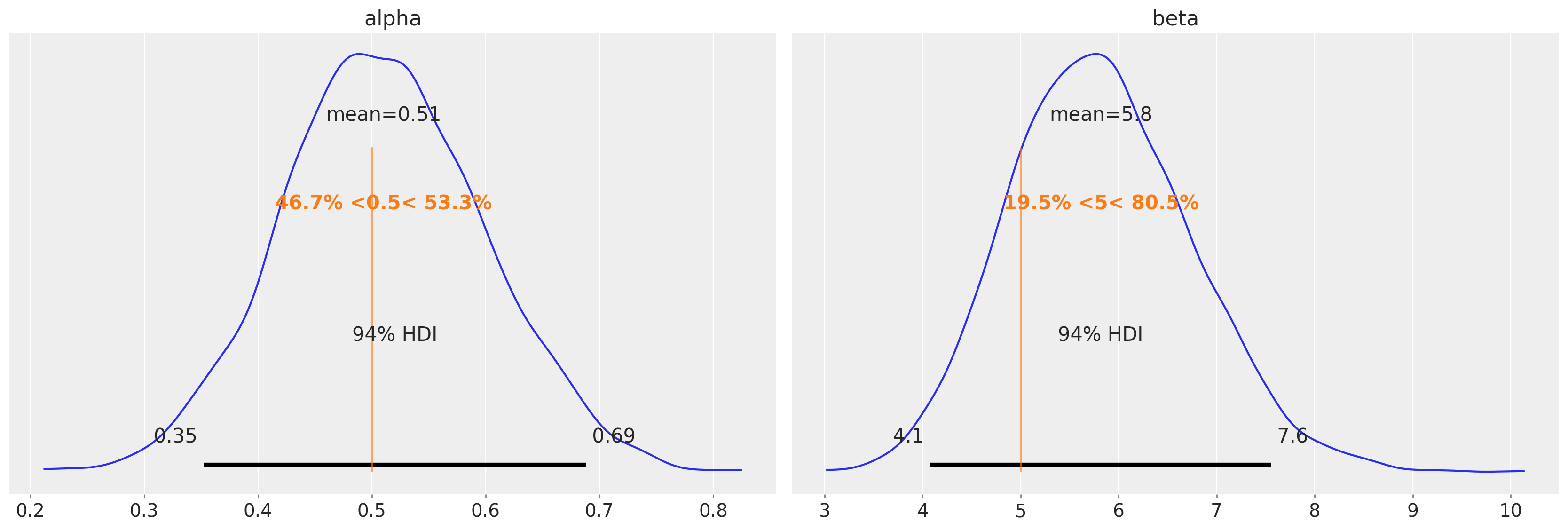
az.plot_posterior(data=tr, ref_val=[true_alpha, true_beta]);

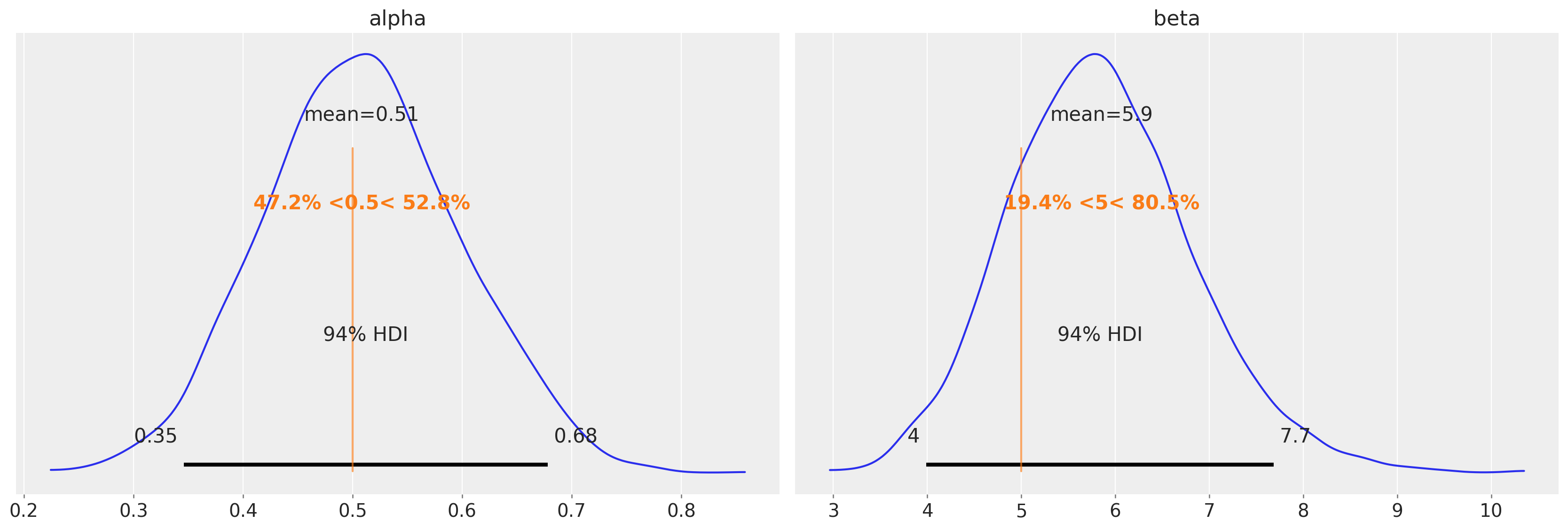
在这个例子中，获得的后验分布很好地集中在最大似然估计值周围。我们得到的是这些值周围合理不确定性的概念。

使用伯努利分布作为似然函数的替代模型

在最后一部分，我提供了一个使用伯努利似然的模型的替代实现。

注意

使用伯努利似然的一个原因是，可以进行先验和后验预测采样以及模型比较。使用 pm.Potential 无法实现这一点，因为 PyMC 不知道什么是似然，什么是先验，也不知道如何生成随机样本。使用 pm.Bernoulli 似然时，这些问题都不存在。

def right_action_probs(alpha, beta, actions, rewards):
    rewards = pt.as_tensor_variable(rewards, dtype="int32")
    actions = pt.as_tensor_variable(actions, dtype="int32")

    # Compute the Qs values
    Qs = 0.5 * pt.ones((2,), dtype="float64")
    Qs, updates = pytensor.scan(
        fn=update_Q, sequences=[actions, rewards], outputs_info=[Qs], non_sequences=[alpha]
    )

    # Apply the sotfmax transformation
    Qs = Qs[:-1] * beta
    logp_actions = Qs - pt.logsumexp(Qs, axis=1, keepdims=True)

    # Return the probabilities for the right action, in the original scale
    return pt.exp(logp_actions[:, 1])

with pm.Model() as m_alt:
    alpha = pm.Beta(name="alpha", alpha=1, beta=1)
    beta = pm.HalfNormal(name="beta", sigma=10)

    action_probs = right_action_probs(alpha, beta, actions, rewards)
    like = pm.Bernoulli(name="like", p=action_probs, observed=actions[1:])

    tr_alt = pm.sample(random_seed=rng)

Auto-assigning NUTS sampler...
Initializing NUTS using jitter+adapt_diag...
Multiprocess sampling (4 chains in 4 jobs)
NUTS: [alpha, beta]

100.00% [8000/8000 00:34<00:00 Sampling 4 chains, 0 divergences]

Sampling 4 chains for 1_000 tune and 1_000 draw iterations (4_000 + 4_000 draws total) took 58 seconds.

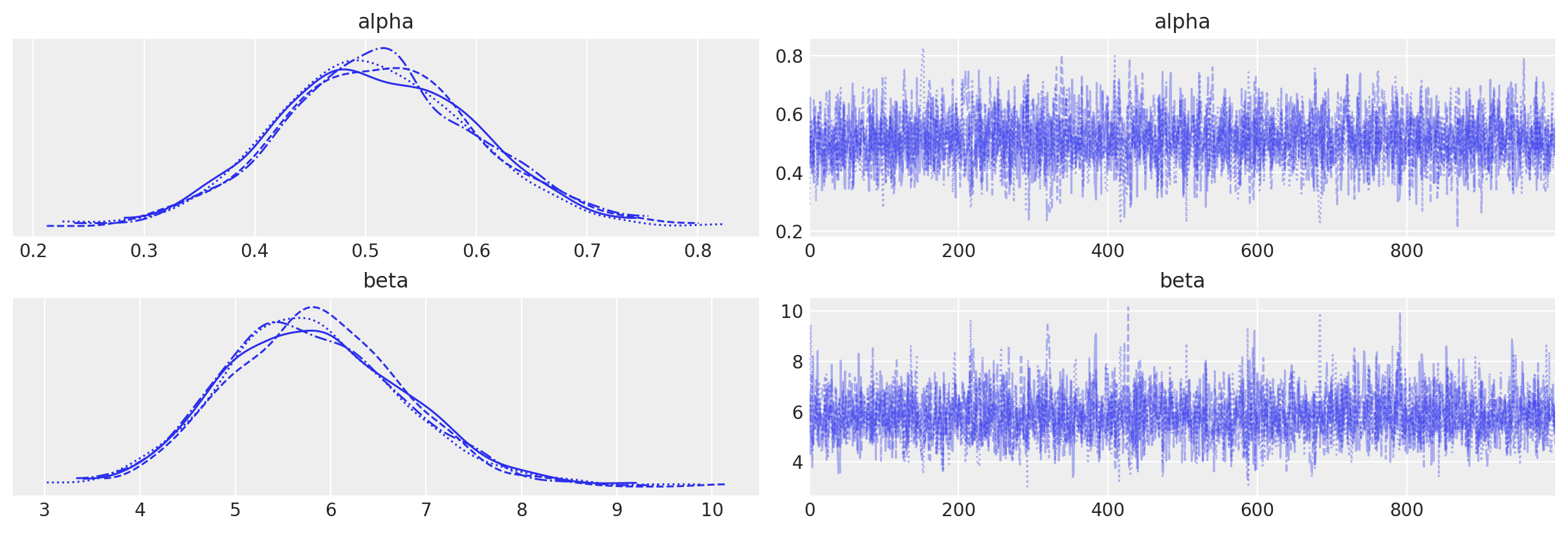
az.plot_trace(data=tr_alt);

az.plot_posterior(data=tr_alt, ref_val=[true_alpha, true_beta]);

水印

%load_ext watermark
%watermark -n -u -v -iv -w -p aeppl,xarray

Last updated: Thu Aug 18 2022

Python implementation: CPython
Python version       : 3.9.13
IPython version      : 8.4.0

aeppl : 0.0.34
xarray: 2022.6.0

pytensor    : 2.7.9
arviz     : 0.12.1
pymc      : 4.1.5
sys       : 3.9.13 (main, May 24 2022, 21:28:31) 
[Clang 13.1.6 (clang-1316.0.21.2)]
scipy     : 1.8.1
numpy     : 1.22.4
matplotlib: 3.5.3

Watermark: 2.3.1

参考资料

[1]

罗伯特·C·威尔逊和安妮·G·E·柯林斯。行为数据计算建模的十个简单规则。eLife，8:e49547，2019年11月。doi:10.7554/eLife.49547。

积分

• 由 Ricardo Vieira 于2022年6月撰写

  • 改编自Maria Eckstein的PyMC代码（GitHub，PyMC讨论区）

  • 改编自Robert Wilson和Anne Collins的MLE代码 [Wilson和Collins, 2019] (GitHub)

• 由 Juan Orduz 于2022年8月重新执行（pymc-examples#410）