


可靠性统计与预测校准#
import os
import random

from io import StringIO

import arviz as az
import matplotlib.cm as cm
import matplotlib.pyplot as plt
import numpy as np
import pandas as pd
import pymc as pm

from lifelines import KaplanMeierFitter, LogNormalFitter, WeibullFitter
from lifelines.utils import survival_table_from_events
from scipy.stats import binom, lognorm, norm, weibull_min
RANDOM_SEED = 8927
rng = np.random.default_rng(RANDOM_SEED)
az.style.use("arviz-darkgrid")
%config InlineBackend.figure_format = 'retina'
可靠性统计#
当我们想要对生产线上的潜在故障进行推断时,我们可能会根据行业、商品性质或我们试图回答的具体问题,拥有大样本或小样本数据集。但在所有情况下,都存在成本问题和可容忍的故障数量。
因此,可靠性研究必须考虑故障发生的重要观察期、故障成本以及运行错误指定研究的成本。在问题的定义和建模练习的性质方面,精确性的要求至关重要。
失效时间数据的关键特征在于其删失方式以及这种删失如何影响传统的统计汇总和估计技术。在本笔记本中,我们将重点放在失效时间的预测上,并将贝叶斯校准预测区间的概念与一些频率主义的替代方法进行比较。我们借鉴了《可靠性数据统计方法》一书中的工作。详情请参见(见 Meeker 等 [2022])
预测的类型#
我们可能想要了解故障时间分布的不同视图,例如:
新产品的故障时间
未来样本中m个单位内发生k次故障的时间
虽然存在非参数和描述性方法可以用于评估这类问题,但我们主要关注的是我们有一个概率模型的情况,例如失效时间的对数正态分布 \(F(t: \mathbf{\theta})\),由未知的 \(\mathbf{\theta}\) 参数化。
演示文稿的结构#
我们将
讨论可靠性数据的累积密度函数CDF的非参数估计
展示如何推导出相同函数的频率主义者或最大似然估计,以指导我们的预测区间
展示贝叶斯方法如何在信息稀疏的情况下用于增强对相同CDF的分析。
在整个过程中,重点将放在理解CDF如何帮助我们在可靠性环境中理解失败风险。特别是如何使用CDF来推导出一个经过良好校准的预测区间。
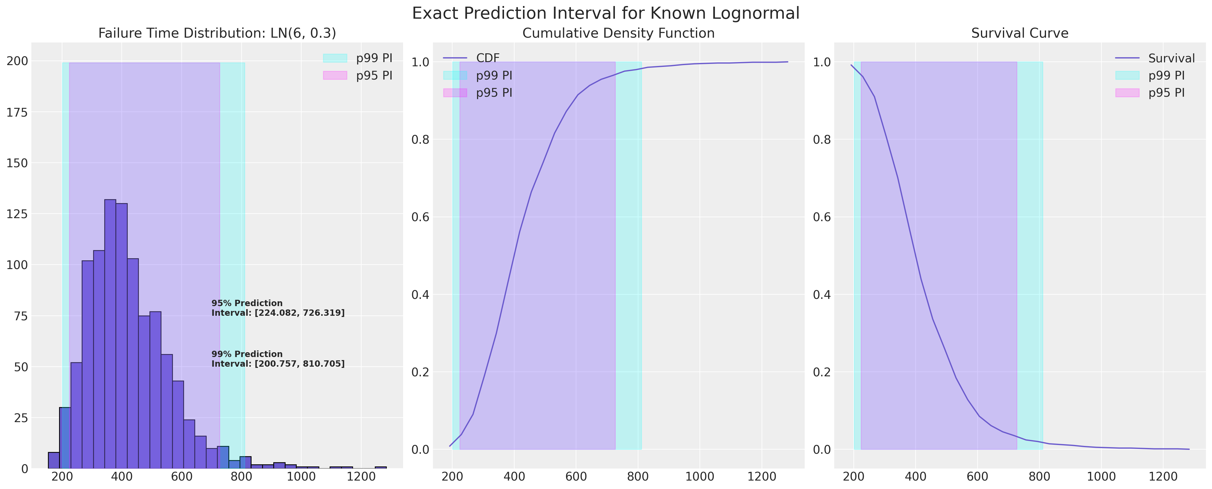
示例失败分布#
在可靠性统计研究中,重点在于具有长尾的位置-尺度分布。在一个理想的世界中,我们会确切知道哪个分布描述了我们的故障过程,并且可以精确地定义下一次故障的预测区间。
mu, sigma = 6, 0.3


def plot_ln_pi(mu, sigma, xy=(700, 75), title="Exact Prediction Interval for Known Lognormal"):
    failure_dist = lognorm(s=sigma, scale=np.exp(mu))
    samples = failure_dist.rvs(size=1000, random_state=100)
    fig, axs = plt.subplots(1, 3, figsize=(20, 8))
    axs = axs.flatten()
    axs[0].hist(samples, ec="black", color="slateblue", bins=30)
    axs[0].set_title(f"Failure Time Distribution: LN({mu}, {sigma})")
    count, bins_count = np.histogram(samples, bins=30)
    pdf = count / sum(count)
    cdf = np.cumsum(pdf)
    axs[1].plot(bins_count[1:], cdf, label="CDF", color="slateblue")
    axs[2].plot(bins_count[1:], 1 - cdf, label="Survival", color="slateblue")
    axs[2].legend()
    axs[1].legend()
    axs[1].set_title("Cumulative Density Function")
    axs[2].set_title("Survival Curve")

    lb = failure_dist.ppf(0.01)
    ub = failure_dist.ppf(0.99)
    axs[0].annotate(
        f"99% Prediction \nInterval: [{np.round(lb, 3)}, {np.round(ub, 3)}]",
        xy=(xy[0], xy[1] - 25),
        fontweight="bold",
    )
    axs[0].fill_betweenx(y=range(200), x1=lb, x2=ub, alpha=0.2, label="p99 PI", color="cyan")
    axs[1].fill_betweenx(y=range(2), x1=lb, x2=ub, alpha=0.2, label="p99 PI", color="cyan")
    axs[2].fill_betweenx(y=range(2), x1=lb, x2=ub, alpha=0.2, label="p99 PI", color="cyan")
    lb = failure_dist.ppf(0.025)
    ub = failure_dist.ppf(0.975)
    axs[0].annotate(
        f"95% Prediction \nInterval: [{np.round(lb, 3)}, {np.round(ub, 3)}]",
        xy=(xy[0], xy[1]),
        fontweight="bold",
    )
    axs[0].fill_betweenx(y=range(200), x1=lb, x2=ub, alpha=0.2, label="p95 PI", color="magenta")
    axs[1].fill_betweenx(y=range(2), x1=lb, x2=ub, alpha=0.2, label="p95 PI", color="magenta")
    axs[2].fill_betweenx(y=range(2), x1=lb, x2=ub, alpha=0.2, label="p95 PI", color="magenta")
    axs[0].legend()
    axs[1].legend()
    axs[2].legend()
    plt.suptitle(title, fontsize=20)


plot_ln_pi(mu, sigma)
从数据中估计故障分布#
在现实世界中,我们很少拥有如此精确的知识。相反,我们通常从完全不那么清晰的数据开始。我们首先将检查三个工厂中关于热交换器的故障数据,并将这些信息汇总起来,以量化这三个工厂中热交换器的使用寿命。
数据是有意设计得较小,以便我们可以专注于评估失效时间数据所涉及的描述性统计。特别是,我们将估计经验累积分布函数和生存函数。然后,我们将这种分析风格推广到更大的数据集之后。
热交换数据#
关于截尾数据的说明: 请参见下文,了解故障数据如何标记一个观测值是否已被截尾,即我们是否已观察到换热器寿命的完整过程。这是故障时间数据的一个重要特征。过于简单的统计汇总会在估计故障发生率时产生偏差,因为我们的研究并未观察到每个项目的完整生命周期。最常见的截尾形式是所谓的“右截尾”数据,其中我们没有观察到部分观测值的“故障”事件。由于过早结束数据收集,我们的历史记录是不完整的。
左删失(我们从其历史记录的开始部分无法观察到某个项目)和区间删失(包括左删失和右删失)也可能发生,但较为少见。
Show code cell source
heat_exchange_df = pd.read_csv(
    StringIO(
        """Years Lower,Years Upper,Censoring Indicator,Count,Plant
0,1,Left,1,1
1,2,Interval,2,1
2,3,Interval,2,1
3, ,Right,95,1
0,1,Left,2,2
1,2,Interval,3,2
2, ,Right,95,2
0,1,Left,1,3
1, ,Right,99,3

"""
    )
)

heat_exchange_df["year_interval"] = (
    heat_exchange_df["Years Lower"].astype(str) + "," + heat_exchange_df["Years Upper"].astype(str)
)
heat_exchange_df["failed"] = np.where(
    heat_exchange_df["Censoring Indicator"] != "Right", heat_exchange_df["Count"], 0
)
heat_exchange_df["censored"] = np.where(
    heat_exchange_df["Censoring Indicator"] == "Right", heat_exchange_df["Count"], 0
)
heat_exchange_df["risk_set"] = [100, 99, 97, 0, 100, 98, 0, 100, 0]
heat_exchange_df
| Years Lower | Years Upper | Censoring Indicator | Count | Plant | year_interval | failed | censored | risk_set | |
|---|---|---|---|---|---|---|---|---|---|
| 0 | 0 | 1 | Left | 1 | 1 | 0,1 | 1 | 0 | 100 |
| 1 | 1 | 2 | Interval | 2 | 1 | 1,2 | 2 | 0 | 99 |
| 2 | 2 | 3 | Interval | 2 | 1 | 2,3 | 2 | 0 | 97 |
| 3 | 3 | Right | 95 | 1 | 3, | 0 | 95 | 0 | |
| 4 | 0 | 1 | Left | 2 | 2 | 0,1 | 2 | 0 | 100 |
| 5 | 1 | 2 | Interval | 3 | 2 | 1,2 | 3 | 0 | 98 |
| 6 | 2 | Right | 95 | 2 | 2, | 0 | 95 | 0 | |
| 7 | 0 | 1 | Left | 1 | 3 | 0,1 | 1 | 0 | 100 |
| 8 | 1 | Right | 99 | 3 | 1, | 0 | 99 | 0 |
actuarial_table = heat_exchange_df.groupby(["Years Upper"])[["failed", "risk_set"]].sum()
actuarial_table = actuarial_table.tail(3)


def greenwood_variance(df):
    ### Used to estimate the variance in the CDF
    n = len(df)
    ps = [df.iloc[i]["p_hat"] / (df.iloc[i]["risk_set"] * df.iloc[i]["1-p_hat"]) for i in range(n)]
    s = [(df.iloc[i]["S_hat"] ** 2) * np.sum(ps[0 : i + 1]) for i in range(n)]
    return s


def logit_transform_interval(df):
    ### Used for robustness in the estimation of the Confidence intervals in the CDF
    df["logit_CI_95_lb"] = df["F_hat"] / (
        df["F_hat"]
        + df["S_hat"] * np.exp((1.960 * df["Standard_Error"]) / (df["F_hat"] * df["S_hat"]))
    )
    df["logit_CI_95_ub"] = df["F_hat"] / (
        df["F_hat"]
        + df["S_hat"] / np.exp((1.960 * df["Standard_Error"]) / (df["F_hat"] * df["S_hat"]))
    )
    df["logit_CI_95_lb"] = np.where(df["logit_CI_95_lb"] < 0, 0, df["logit_CI_95_lb"])
    df["logit_CI_95_ub"] = np.where(df["logit_CI_95_ub"] > 1, 1, df["logit_CI_95_ub"])
    return df


def make_actuarial_table(actuarial_table):
    ### Actuarial lifetables are used to describe the nature of the risk over time and estimate
    actuarial_table["p_hat"] = actuarial_table["failed"] / actuarial_table["risk_set"]
    actuarial_table["1-p_hat"] = 1 - actuarial_table["p_hat"]
    actuarial_table["S_hat"] = actuarial_table["1-p_hat"].cumprod()
    actuarial_table["CH_hat"] = -np.log(actuarial_table["S_hat"])
    ### The Estimate of the CDF function
    actuarial_table["F_hat"] = 1 - actuarial_table["S_hat"]
    actuarial_table["V_hat"] = greenwood_variance(actuarial_table)
    actuarial_table["Standard_Error"] = np.sqrt(actuarial_table["V_hat"])
    actuarial_table["CI_95_lb"] = (
        actuarial_table["F_hat"] - actuarial_table["Standard_Error"] * 1.960
    )
    actuarial_table["CI_95_lb"] = np.where(
        actuarial_table["CI_95_lb"] < 0, 0, actuarial_table["CI_95_lb"]
    )
    actuarial_table["CI_95_ub"] = (
        actuarial_table["F_hat"] + actuarial_table["Standard_Error"] * 1.960
    )
    actuarial_table["CI_95_ub"] = np.where(
        actuarial_table["CI_95_ub"] > 1, 1, actuarial_table["CI_95_ub"]
    )
    actuarial_table["ploting_position"] = actuarial_table["F_hat"].rolling(1).median()
    actuarial_table = logit_transform_interval(actuarial_table)
    return actuarial_table


actuarial_table_heat = make_actuarial_table(actuarial_table)
actuarial_table_heat = actuarial_table_heat.reset_index()
actuarial_table_heat.rename({"Years Upper": "t"}, axis=1, inplace=True)
actuarial_table_heat["t"] = actuarial_table_heat["t"].astype(int)
actuarial_table_heat
| t | failed | risk_set | p_hat | 1-p_hat | S_hat | CH_hat | F_hat | V_hat | Standard_Error | CI_95_lb | CI_95_ub | ploting_position | logit_CI_95_lb | logit_CI_95_ub | |
|---|---|---|---|---|---|---|---|---|---|---|---|---|---|---|---|
| 0 | 1 | 4 | 300 | 0.013333 | 0.986667 | 0.986667 | 0.013423 | 0.013333 | 0.000044 | 0.006622 | 0.000354 | 0.026313 | 0.013333 | 0.005013 | 0.034977 |
| 1 | 2 | 5 | 197 | 0.025381 | 0.974619 | 0.961624 | 0.039131 | 0.038376 | 0.000164 | 0.012802 | 0.013283 | 0.063468 | 0.038376 | 0.019818 | 0.073016 |
| 2 | 3 | 2 | 97 | 0.020619 | 0.979381 | 0.941797 | 0.059965 | 0.058203 | 0.000350 | 0.018701 | 0.021550 | 0.094856 | 0.058203 | 0.030694 | 0.107629 |
值得花一些时间来详细讲解这个例子,因为它建立了时间到故障模型中一些关键量的估计。
首先注意我们如何将时间视为一系列离散的时间间隔。数据格式是离散的周期格式,因为它记录了随时间的累计故障。我们将在下面看到另一种故障数据格式——项目-周期格式,它记录了所有周期内的每个单独项目及其对应的状态。在这种格式中,关键量是每个周期内的failed项目集和risk_set。其他所有内容都由此推导而来。
首先,我们在连续三年的三个公司中确定了生产的热交换器的数量及其随后失败的数量。这提供了当年失败概率的估计值:p_hat 及其逆值 1-p_hat。这些值在一年中进一步结合,以估计生存曲线 S_hat,该曲线可以进一步转换以恢复累积危险 CH_hat 和累积密度函数 F_hat 的估计值。
接下来,我们希望有一种快速且粗略的方法来量化我们对CDF估计的不确定性程度。为此,我们使用greenwood公式来估计我们估计的V_hat的方差,即F_hat。这为我们提供了标准误差以及文献中推荐的两类置信区间。
我们将相同的技术应用于更大的数据集,并在下面绘制了一些这些量。
减震器数据:频繁主义可靠性分析研究#
减震器数据采用周期格式,但它记录了随着时间推移风险集不断减少的情况,即在每个时间点有一个项目被删失或失效,即从测试中成功移除(通过)或因失效而移除。这是周期格式数据的特殊情况。
Show code cell source
shockabsorbers_df = pd.read_csv(
    StringIO(
        """Kilometers,Failure Mode,Censoring Indicator
6700,Mode1,Failed
6950,Censored,Censored
7820,Censored,Censored
8790,Censored,Censored
9120,Mode2,Failed
9660,Censored,Censored
9820,Censored,Censored
11310,Censored,Censored
11690,Censored,Censored
11850,Censored,Censored
11880,Censored,Censored
12140,Censored,Censored
12200,Mode1,Failed
12870,Censored,Censored
13150,Mode2,Failed
13330,Censored,Censored
13470,Censored,Censored
14040,Censored,Censored
14300,Mode1,Failed
17520,Mode1,Failed
17540,Censored,Censored
17890,Censored,Censored
18450,Censored,Censored
18960,Censored,Censored
18980,Censored,Censored
19410,Censored,Censored
20100,Mode2,Failed
20100,Censored,Censored
20150,Censored,Censored
20320,Censored,Censored
20900,Mode2,Failed
22700,Mode1,Failed
23490,Censored,Censored
26510,Mode1,Failed
27410,Censored,Censored
27490,Mode1,Failed
27890,Censored,Censored
28100,Censored,Censored
"""
    )
)

shockabsorbers_df["failed"] = np.where(shockabsorbers_df["Censoring Indicator"] == "Failed", 1, 0)
shockabsorbers_df["t"] = shockabsorbers_df["Kilometers"]
shockabsorbers_events = survival_table_from_events(
    shockabsorbers_df["t"], shockabsorbers_df["failed"]
).reset_index()
shockabsorbers_events.rename(
    {"event_at": "t", "observed": "failed", "at_risk": "risk_set"}, axis=1, inplace=True
)
actuarial_table_shock = make_actuarial_table(shockabsorbers_events)
actuarial_table_shock
| t | removed | failed | censored | entrance | risk_set | p_hat | 1-p_hat | S_hat | CH_hat | F_hat | V_hat | Standard_Error | CI_95_lb | CI_95_ub | ploting_position | logit_CI_95_lb | logit_CI_95_ub | |
|---|---|---|---|---|---|---|---|---|---|---|---|---|---|---|---|---|---|---|
| 0 | 0.0 | 0 | 0 | 0 | 38 | 38 | 0.000000 | 1.000000 | 1.000000 | -0.000000 | 0.000000 | 0.000000 | 0.000000 | 0.000000 | 0.000000 | 0.000000 | NaN | NaN |
| 1 | 6700.0 | 1 | 1 | 0 | 0 | 38 | 0.026316 | 0.973684 | 0.973684 | 0.026668 | 0.026316 | 0.000674 | 0.025967 | 0.000000 | 0.077212 | 0.026316 | 0.003694 | 0.164570 |
| 2 | 6950.0 | 1 | 0 | 1 | 0 | 37 | 0.000000 | 1.000000 | 0.973684 | 0.026668 | 0.026316 | 0.000674 | 0.025967 | 0.000000 | 0.077212 | 0.026316 | 0.003694 | 0.164570 |
| 3 | 7820.0 | 1 | 0 | 1 | 0 | 36 | 0.000000 | 1.000000 | 0.973684 | 0.026668 | 0.026316 | 0.000674 | 0.025967 | 0.000000 | 0.077212 | 0.026316 | 0.003694 | 0.164570 |
| 4 | 8790.0 | 1 | 0 | 1 | 0 | 35 | 0.000000 | 1.000000 | 0.973684 | 0.026668 | 0.026316 | 0.000674 | 0.025967 | 0.000000 | 0.077212 | 0.026316 | 0.003694 | 0.164570 |
| 5 | 9120.0 | 1 | 1 | 0 | 0 | 34 | 0.029412 | 0.970588 | 0.945046 | 0.056521 | 0.054954 | 0.001431 | 0.037831 | 0.000000 | 0.129103 | 0.054954 | 0.013755 | 0.195137 |
| 6 | 9660.0 | 1 | 0 | 1 | 0 | 33 | 0.000000 | 1.000000 | 0.945046 | 0.056521 | 0.054954 | 0.001431 | 0.037831 | 0.000000 | 0.129103 | 0.054954 | 0.013755 | 0.195137 |
| 7 | 9820.0 | 1 | 0 | 1 | 0 | 32 | 0.000000 | 1.000000 | 0.945046 | 0.056521 | 0.054954 | 0.001431 | 0.037831 | 0.000000 | 0.129103 | 0.054954 | 0.013755 | 0.195137 |
| 8 | 11310.0 | 1 | 0 | 1 | 0 | 31 | 0.000000 | 1.000000 | 0.945046 | 0.056521 | 0.054954 | 0.001431 | 0.037831 | 0.000000 | 0.129103 | 0.054954 | 0.013755 | 0.195137 |
| 9 | 11690.0 | 1 | 0 | 1 | 0 | 30 | 0.000000 | 1.000000 | 0.945046 | 0.056521 | 0.054954 | 0.001431 | 0.037831 | 0.000000 | 0.129103 | 0.054954 | 0.013755 | 0.195137 |
| 10 | 11850.0 | 1 | 0 | 1 | 0 | 29 | 0.000000 | 1.000000 | 0.945046 | 0.056521 | 0.054954 | 0.001431 | 0.037831 | 0.000000 | 0.129103 | 0.054954 | 0.013755 | 0.195137 |
| 11 | 11880.0 | 1 | 0 | 1 | 0 | 28 | 0.000000 | 1.000000 | 0.945046 | 0.056521 | 0.054954 | 0.001431 | 0.037831 | 0.000000 | 0.129103 | 0.054954 | 0.013755 | 0.195137 |
| 12 | 12140.0 | 1 | 0 | 1 | 0 | 27 | 0.000000 | 1.000000 | 0.945046 | 0.056521 | 0.054954 | 0.001431 | 0.037831 | 0.000000 | 0.129103 | 0.054954 | 0.013755 | 0.195137 |
| 13 | 12200.0 | 1 | 1 | 0 | 0 | 26 | 0.038462 | 0.961538 | 0.908698 | 0.095742 | 0.091302 | 0.002594 | 0.050927 | 0.000000 | 0.191119 | 0.091302 | 0.029285 | 0.250730 |
| 14 | 12870.0 | 1 | 0 | 1 | 0 | 25 | 0.000000 | 1.000000 | 0.908698 | 0.095742 | 0.091302 | 0.002594 | 0.050927 | 0.000000 | 0.191119 | 0.091302 | 0.029285 | 0.250730 |
| 15 | 13150.0 | 1 | 1 | 0 | 0 | 24 | 0.041667 | 0.958333 | 0.870836 | 0.138302 | 0.129164 | 0.003756 | 0.061285 | 0.009046 | 0.249282 | 0.129164 | 0.048510 | 0.301435 |
| 16 | 13330.0 | 1 | 0 | 1 | 0 | 23 | 0.000000 | 1.000000 | 0.870836 | 0.138302 | 0.129164 | 0.003756 | 0.061285 | 0.009046 | 0.249282 | 0.129164 | 0.048510 | 0.301435 |
| 17 | 13470.0 | 1 | 0 | 1 | 0 | 22 | 0.000000 | 1.000000 | 0.870836 | 0.138302 | 0.129164 | 0.003756 | 0.061285 | 0.009046 | 0.249282 | 0.129164 | 0.048510 | 0.301435 |
| 18 | 14040.0 | 1 | 0 | 1 | 0 | 21 | 0.000000 | 1.000000 | 0.870836 | 0.138302 | 0.129164 | 0.003756 | 0.061285 | 0.009046 | 0.249282 | 0.129164 | 0.048510 | 0.301435 |
| 19 | 14300.0 | 1 | 1 | 0 | 0 | 20 | 0.050000 | 0.950000 | 0.827294 | 0.189595 | 0.172706 | 0.005191 | 0.072047 | 0.031495 | 0.313917 | 0.172706 | 0.072098 | 0.359338 |
| 20 | 17520.0 | 1 | 1 | 0 | 0 | 19 | 0.052632 | 0.947368 | 0.783752 | 0.243662 | 0.216248 | 0.006455 | 0.080342 | 0.058778 | 0.373717 | 0.216248 | 0.098254 | 0.411308 |
| 21 | 17540.0 | 1 | 0 | 1 | 0 | 18 | 0.000000 | 1.000000 | 0.783752 | 0.243662 | 0.216248 | 0.006455 | 0.080342 | 0.058778 | 0.373717 | 0.216248 | 0.098254 | 0.411308 |
| 22 | 17890.0 | 1 | 0 | 1 | 0 | 17 | 0.000000 | 1.000000 | 0.783752 | 0.243662 | 0.216248 | 0.006455 | 0.080342 | 0.058778 | 0.373717 | 0.216248 | 0.098254 | 0.411308 |
| 23 | 18450.0 | 1 | 0 | 1 | 0 | 16 | 0.000000 | 1.000000 | 0.783752 | 0.243662 | 0.216248 | 0.006455 | 0.080342 | 0.058778 | 0.373717 | 0.216248 | 0.098254 | 0.411308 |
| 24 | 18960.0 | 1 | 0 | 1 | 0 | 15 | 0.000000 | 1.000000 | 0.783752 | 0.243662 | 0.216248 | 0.006455 | 0.080342 | 0.058778 | 0.373717 | 0.216248 | 0.098254 | 0.411308 |
| 25 | 18980.0 | 1 | 0 | 1 | 0 | 14 | 0.000000 | 1.000000 | 0.783752 | 0.243662 | 0.216248 | 0.006455 | 0.080342 | 0.058778 | 0.373717 | 0.216248 | 0.098254 | 0.411308 |
| 26 | 19410.0 | 1 | 0 | 1 | 0 | 13 | 0.000000 | 1.000000 | 0.783752 | 0.243662 | 0.216248 | 0.006455 | 0.080342 | 0.058778 | 0.373717 | 0.216248 | 0.098254 | 0.411308 |
| 27 | 20100.0 | 2 | 1 | 1 | 0 | 12 | 0.083333 | 0.916667 | 0.718440 | 0.330673 | 0.281560 | 0.009334 | 0.096613 | 0.092199 | 0.470922 | 0.281560 | 0.133212 | 0.499846 |
| 28 | 20150.0 | 1 | 0 | 1 | 0 | 10 | 0.000000 | 1.000000 | 0.718440 | 0.330673 | 0.281560 | 0.009334 | 0.096613 | 0.092199 | 0.470922 | 0.281560 | 0.133212 | 0.499846 |
| 29 | 20320.0 | 1 | 0 | 1 | 0 | 9 | 0.000000 | 1.000000 | 0.718440 | 0.330673 | 0.281560 | 0.009334 | 0.096613 | 0.092199 | 0.470922 | 0.281560 | 0.133212 | 0.499846 |
| 30 | 20900.0 | 1 | 1 | 0 | 0 | 8 | 0.125000 | 0.875000 | 0.628635 | 0.464205 | 0.371365 | 0.014203 | 0.119177 | 0.137778 | 0.604953 | 0.371365 | 0.178442 | 0.616380 |
| 31 | 22700.0 | 1 | 1 | 0 | 0 | 7 | 0.142857 | 0.857143 | 0.538830 | 0.618356 | 0.461170 | 0.017348 | 0.131711 | 0.203016 | 0.719324 | 0.461170 | 0.232453 | 0.707495 |
| 32 | 23490.0 | 1 | 0 | 1 | 0 | 6 | 0.000000 | 1.000000 | 0.538830 | 0.618356 | 0.461170 | 0.017348 | 0.131711 | 0.203016 | 0.719324 | 0.461170 | 0.232453 | 0.707495 |
| 33 | 26510.0 | 1 | 1 | 0 | 0 | 5 | 0.200000 | 0.800000 | 0.431064 | 0.841499 | 0.568936 | 0.020393 | 0.142806 | 0.289037 | 0.848835 | 0.568936 | 0.296551 | 0.805150 |
| 34 | 27410.0 | 1 | 0 | 1 | 0 | 4 | 0.000000 | 1.000000 | 0.431064 | 0.841499 | 0.568936 | 0.020393 | 0.142806 | 0.289037 | 0.848835 | 0.568936 | 0.296551 | 0.805150 |
| 35 | 27490.0 | 1 | 1 | 0 | 0 | 3 | 0.333333 | 0.666667 | 0.287376 | 1.246964 | 0.712624 | 0.022828 | 0.151089 | 0.416490 | 1.000000 | 0.712624 | 0.368683 | 0.913267 |
| 36 | 27890.0 | 1 | 0 | 1 | 0 | 2 | 0.000000 | 1.000000 | 0.287376 | 1.246964 | 0.712624 | 0.022828 | 0.151089 | 0.416490 | 1.000000 | 0.712624 | 0.368683 | 0.913267 |
| 37 | 28100.0 | 1 | 0 | 1 | 0 | 1 | 0.000000 | 1.000000 | 0.287376 | 1.246964 | 0.712624 | 0.022828 | 0.151089 | 0.416490 | 1.000000 | 0.712624 | 0.368683 | 0.913267 |
故障数据的极大似然拟合#
除了对我们的数据进行描述性总结外,我们还可以使用生命表数据来估计一个适合我们故障时间分布的单变量模型。如果拟合良好,这将使我们能够更清晰地了解特定预测区间的预测分布。在这里,我们将使用 lifelines 包中的函数来估计右删失数据的极大似然拟合。
lnf = LogNormalFitter().fit(actuarial_table_shock["t"] + 1e-25, actuarial_table_shock["failed"])
lnf.print_summary()
| model | lifelines.LogNormalFitter |
|---|---|
| number of observations | 38 |
| number of events observed | 11 |
| log-likelihood | -124.20 |
| hypothesis | mu_ != 0, sigma_ != 1 |
| coef | se(coef) | coef lower 95% | coef upper 95% | cmp to | z | p | -log2(p) | |
|---|---|---|---|---|---|---|---|---|
| mu_ | 10.13 | 0.14 | 9.85 | 10.41 | 0.00 | 71.08 | <0.005 | inf |
| sigma_ | 0.53 | 0.11 | 0.31 | 0.74 | 1.00 | -4.26 | <0.005 | 15.58 |
| AIC | 252.41 |
|---|
尽管我们很想采用这个模型并直接应用,但在数据有限的情况下我们需要谨慎。例如,在热交换数据中,我们有三年的数据,总共只有11次故障。一个过于简单的模型可能会导致错误的结论。目前,我们将专注于减震器数据——其非参数描述以及对该数据的简单单变量拟合。
Show code cell source
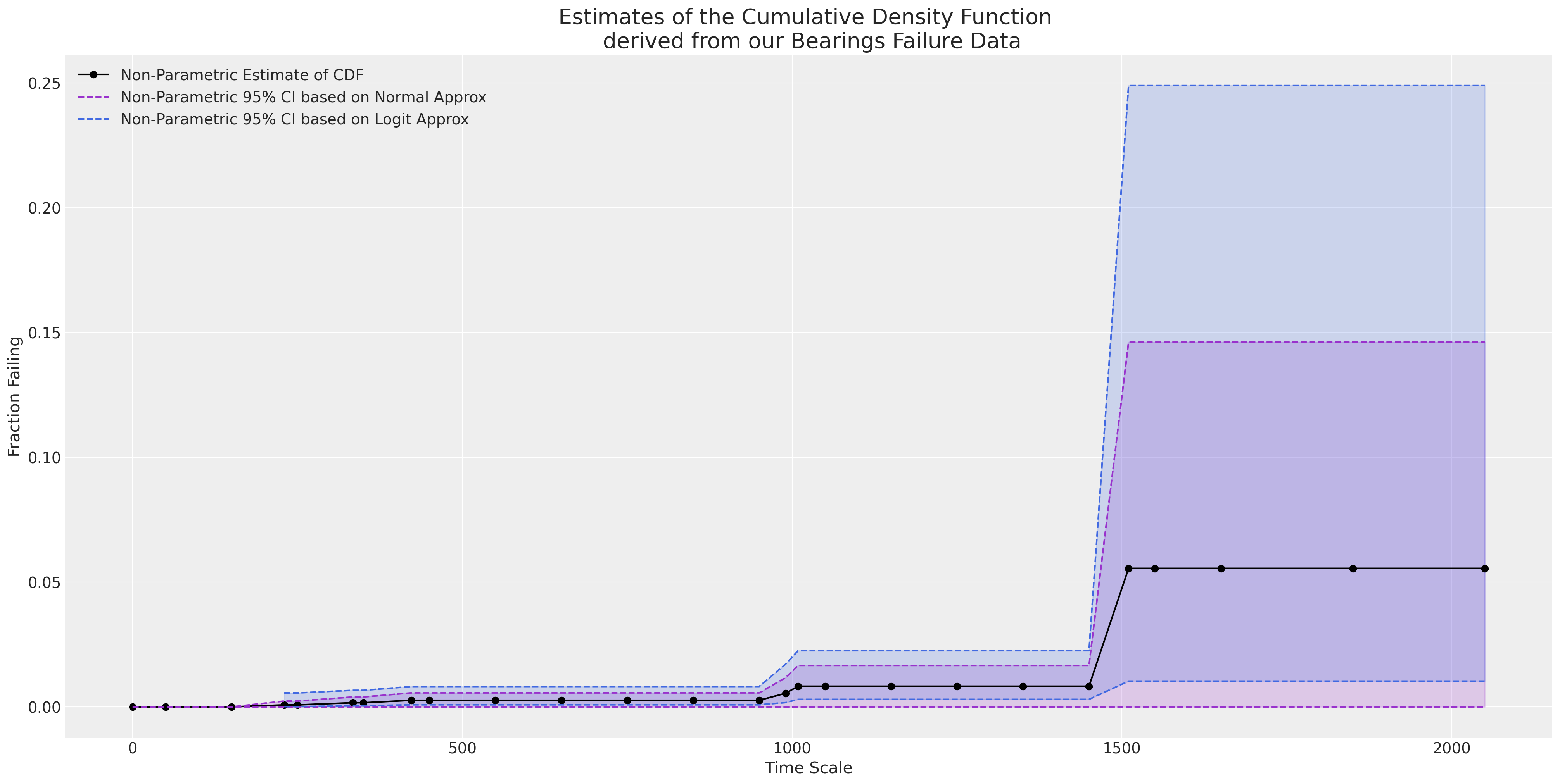
def plot_cdfs(actuarial_table, dist_fits=True, ax=None, title="", xy=(3000, 0.5), item_period=None):
    if item_period is None:
        lnf = LogNormalFitter().fit(actuarial_table["t"] + 1e-25, actuarial_table["failed"])
        wbf = WeibullFitter().fit(actuarial_table["t"] + 1e-25, actuarial_table["failed"])
    else:
        lnf = LogNormalFitter().fit(item_period["t"] + 1e-25, item_period["failed"])
        wbf = WeibullFitter().fit(item_period["t"] + 1e-25, item_period["failed"])
    if ax is None:
        fig, ax = plt.subplots(figsize=(20, 10))
    ax.plot(
        actuarial_table["t"],
        actuarial_table["F_hat"],
        "-o",
        color="black",
        label="Non-Parametric Estimate of CDF",
    )
    ax.plot(
        actuarial_table["t"],
        actuarial_table["CI_95_lb"],
        color="darkorchid",
        linestyle="--",
        label="Non-Parametric 95% CI based on Normal Approx",
    )
    ax.plot(actuarial_table["t"], actuarial_table["CI_95_ub"], color="darkorchid", linestyle="--")
    ax.fill_between(
        actuarial_table["t"].values,
        actuarial_table["CI_95_lb"].values,
        actuarial_table["CI_95_ub"].values,
        color="darkorchid",
        alpha=0.2,
    )
    ax.plot(
        actuarial_table["t"],
        actuarial_table["logit_CI_95_lb"],
        color="royalblue",
        linestyle="--",
        label="Non-Parametric 95% CI based on Logit Approx",
    )
    ax.plot(
        actuarial_table["t"], actuarial_table["logit_CI_95_ub"], color="royalblue", linestyle="--"
    )
    ax.fill_between(
        actuarial_table["t"].values,
        actuarial_table["logit_CI_95_lb"].values,
        actuarial_table["logit_CI_95_ub"].values,
        color="royalblue",
        alpha=0.2,
    )
    if dist_fits:
        lnf.plot_cumulative_density(ax=ax, color="crimson", alpha=0.8)
        wbf.plot_cumulative_density(ax=ax, color="cyan", alpha=0.8)
        ax.annotate(
            f"Lognormal Fit: mu = {np.round(lnf.mu_, 3)}, sigma = {np.round(lnf.sigma_, 3)} \nWeibull Fit: lambda = {np.round(wbf.lambda_, 3)}, rho = {np.round(wbf.rho_, 3)}",
            xy=(xy[0], xy[1]),
            fontsize=12,
            weight="bold",
        )
    ax.set_title(
        f"Estimates of the Cumulative Density Function \n derived from our {title} Failure Data",
        fontsize=20,
    )
    ax.set_ylabel("Fraction Failing")
    ax.set_xlabel("Time Scale")
    ax.legend()
    return ax
plot_cdfs(actuarial_table_shock, title="Shock Absorber");
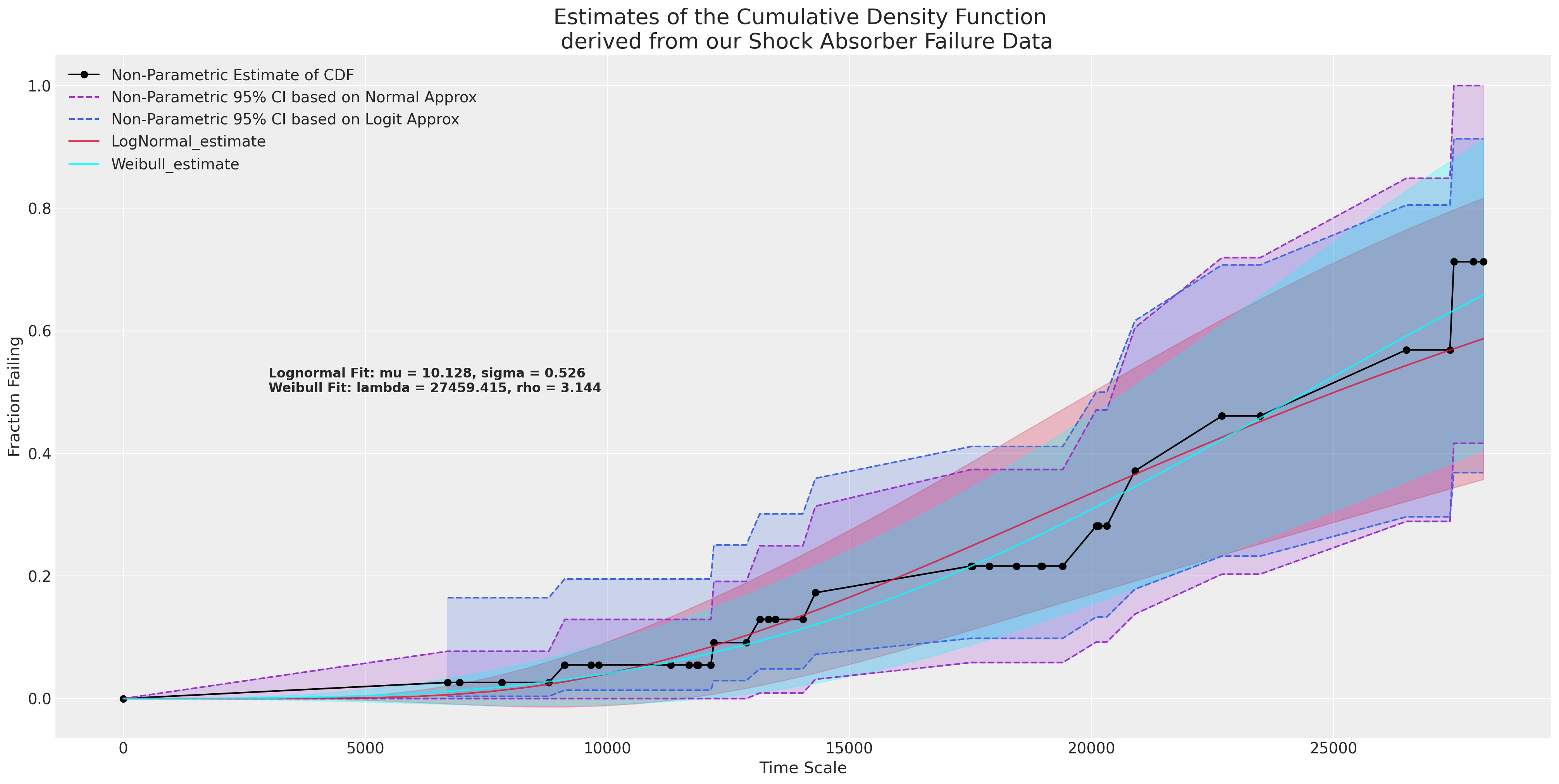
这表明与数据的拟合良好,并且正如您可能预期的那样,随着减震器的老化,失效的比例会增加。但是,我们如何量化给定估计模型的预测呢?
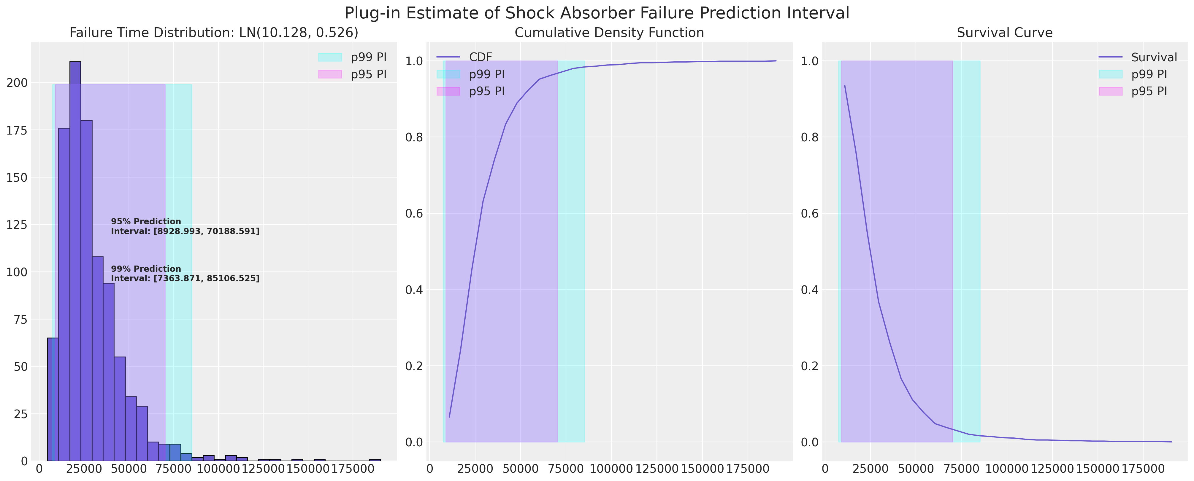
计算近似统计预测区间的插件程序#
由于我们已经估计了减震器数据CDF的对数正态拟合,我们可以绘制其近似的预测区间。这里可能感兴趣的是预测区间的下限,因为作为制造商,我们可能希望了解保修索赔以及如果下限过低,面临退款风险的情况。
plot_ln_pi(
    10.128,
    0.526,
    xy=(40000, 120),
    title="Plug-in Estimate of Shock Absorber Failure Prediction Interval",
)
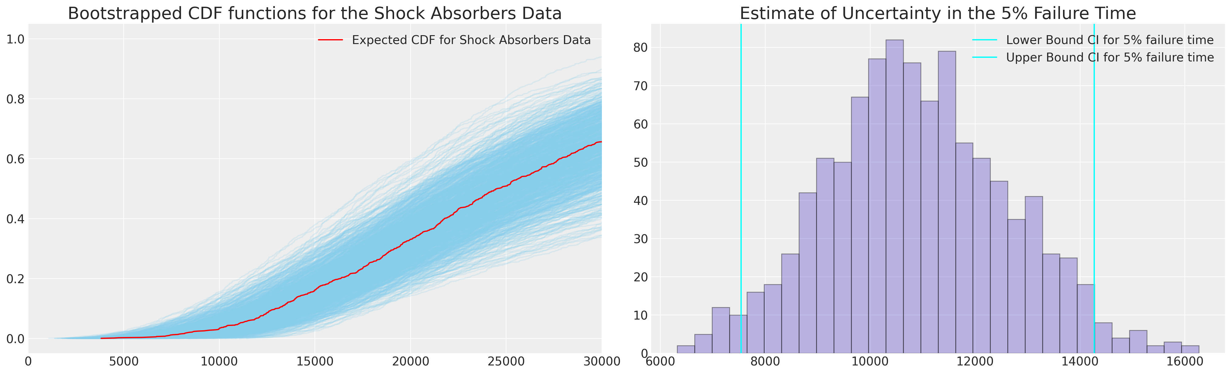
Bootstrap校准与覆盖估计#
我们现在想要估计这个预测区间所隐含的覆盖率,为此我们将对95%置信区间的上下界进行自举估计,并最终评估它们在最大似然估计(MLE)拟合条件下的覆盖率。我们将使用分数加权(贝叶斯)自举法。我们将报告两种估计覆盖率统计量的方法——第一种是基于从已知范围内随机抽取一个值,并评估它是否落在95% MLE的上下界之间。
我们评估覆盖率的第二种方法是引导估计95%的下限和上限,然后评估这些引导值在最大似然估计(MLE)拟合条件下覆盖的范围。
def bayes_boot(df, lb, ub, seed=100):
    w = np.random.dirichlet(np.ones(len(df)), 1)[0]
    lnf = LogNormalFitter().fit(df["t"] + 1e-25, df["failed"], weights=w)
    rv = lognorm(s=lnf.sigma_, scale=np.exp(lnf.mu_))
    ## Sample random choice from implied bootstrapped distribution
    choices = rv.rvs(1000)
    future = random.choice(choices)
    ## Check if choice is contained within the MLE 95% PI
    contained = (future >= lb) & (future <= ub)
    ## Record 95% interval of bootstrapped dist
    lb = rv.ppf(0.025)
    ub = rv.ppf(0.975)
    return lb, ub, contained, future, lnf.sigma_, lnf.mu_
CIs = [bayes_boot(actuarial_table_shock, 8928, 70188, seed=i) for i in range(1000)]
draws = pd.DataFrame(
    CIs, columns=["Lower Bound PI", "Upper Bound PI", "Contained", "future", "Sigma", "Mu"]
)
draws
| Lower Bound PI | Upper Bound PI | Contained | future | Sigma | Mu | |
|---|---|---|---|---|---|---|
| 0 | 9539.612509 | 52724.144855 | True | 12721.873679 | 0.436136 | 10.018018 |
| 1 | 11190.287884 | 70193.514908 | True | 37002.708820 | 0.468429 | 10.240906 |
| 2 | 12262.816075 | 49883.853578 | True | 47419.786326 | 0.357947 | 10.115890 |
| 3 | 10542.933491 | 119175.518677 | False | 82191.111953 | 0.618670 | 10.475782 |
| 4 | 9208.478350 | 62352.752208 | True | 25393.072528 | 0.487938 | 10.084221 |
| ... | ... | ... | ... | ... | ... | ... |
| 995 | 9591.084003 | 85887.280659 | True | 53836.013839 | 0.559245 | 10.264690 |
| 996 | 9724.522689 | 45044.965713 | True | 19481.035376 | 0.391081 | 9.948911 |
| 997 | 8385.673724 | 104222.628035 | True | 16417.930907 | 0.642870 | 10.294282 |
| 998 | 11034.708453 | 56492.385175 | True | 42085.798578 | 0.416605 | 10.125331 |
| 999 | 9408.619310 | 51697.495907 | True | 19253.676200 | 0.434647 | 10.001273 |
1000行 × 6列
我们可以使用这些引导统计量来进一步计算预测分布的量。在我们的例子中,我们可以使用简单参数模型的参数CDF,但我们将采用经验CDF来说明当模型更复杂时如何使用这种技术。
def ecdf(sample):
    # convert sample to a numpy array, if it isn't already
    sample = np.atleast_1d(sample)

    # find the unique values and their corresponding counts
    quantiles, counts = np.unique(sample, return_counts=True)

    # take the cumulative sum of the counts and divide by the sample size to
    # get the cumulative probabilities between 0 and 1
    cumprob = np.cumsum(counts).astype(np.double) / sample.size

    return quantiles, cumprob


fig, axs = plt.subplots(1, 2, figsize=(20, 6))
axs = axs.flatten()
ax = axs[0]
ax1 = axs[1]
hist_data = []
for i in range(1000):
    samples = lognorm(s=draws.iloc[i]["Sigma"], scale=np.exp(draws.iloc[i]["Mu"])).rvs(1000)
    qe, pe = ecdf(samples)
    ax.plot(qe, pe, color="skyblue", alpha=0.2)
    lkup = dict(zip(pe, qe))
    hist_data.append([lkup[0.05]])
hist_data = pd.DataFrame(hist_data, columns=["p05"])
samples = lognorm(s=draws["Sigma"].mean(), scale=np.exp(draws["Mu"].mean())).rvs(1000)
qe, pe = ecdf(samples)
ax.plot(qe, pe, color="red", label="Expected CDF for Shock Absorbers Data")
ax.set_xlim(0, 30_000)
ax.set_title("Bootstrapped CDF functions for the Shock Absorbers Data", fontsize=20)
ax1.hist(hist_data["p05"], color="slateblue", ec="black", alpha=0.4, bins=30)
ax1.set_title("Estimate of Uncertainty in the 5% Failure Time", fontsize=20)
ax1.axvline(
    hist_data["p05"].quantile(0.025), color="cyan", label="Lower Bound CI for 5% failure time"
)
ax1.axvline(
    hist_data["p05"].quantile(0.975), color="cyan", label="Upper Bound CI for 5% failure time"
)
ax1.legend()
ax.legend();
接下来我们将绘制自举数据以及基于MLE拟合所达到的两个覆盖率估计。换句话说,当我们想要评估基于MLE拟合的预测区间的覆盖率时,我们也可以自举估计这个量。
Show code cell source
mosaic = """AABB
            CCCC"""
fig, axs = plt.subplot_mosaic(mosaic=mosaic, figsize=(20, 12))
mle_rv = lognorm(s=0.53, scale=np.exp(10.128))
axs = [axs[k] for k in axs.keys()]
axs[0].scatter(
    draws["Mu"],
    draws["Lower Bound PI"],
    c=draws["Contained"],
    cmap=cm.cool,
    alpha=0.3,
    label="Fits in MLE 95% CI",
)
axs[1].scatter(
    draws["Sigma"],
    draws["Lower Bound PI"],
    c=draws["Contained"],
    cmap=cm.cool,
    alpha=0.3,
    label="Fits in MLE 95% CI",
)
axs[0].set_title("Bootstrapped Mu against Bootstrapped 95% Lower Bound")
prop = draws["Contained"].sum() / len(draws)
axs[0].annotate(
    f"Estimated Prediction \nEmpirical Coverage \nBased on Sampling : {np.round(prop, 3)}",
    xy=(10.4, 12000),
    fontweight="bold",
)
axs[1].set_title("Bootstrapped Sigma against Bootstrapped 95% Lower Bound")
axs[0].legend()
axs[0].set_xlabel("Mu")
axs[1].set_xlabel("Sigma")
axs[0].set_ylabel("Estimated Lower 95% PI")
axs[1].legend()
axs[2].hist(
    mle_rv.cdf(draws["Lower Bound PI"]),
    bins=50,
    label="Bootstrap 95% LB",
    ec="k",
    color="royalblue",
    alpha=0.2,
)
axs[2].hist(
    mle_rv.cdf(draws["Upper Bound PI"]),
    bins=50,
    label="Bootstrap 95% UB",
    ec="k",
    color="darkorchid",
    alpha=0.2,
)
axs[2].hist(
    np.abs(mle_rv.cdf(draws["Lower Bound PI"]) - mle_rv.cdf(draws["Upper Bound PI"])),
    alpha=0.2,
    bins=50,
    color="slateblue",
    ec="black",
    label="Bootstrap Abs Diff",
)
axs[2].axvline(
    np.abs(mle_rv.cdf(draws["Lower Bound PI"]) - mle_rv.cdf(draws["Upper Bound PI"])).mean(),
    label="Expected Coverage",
)
axs[2].set_title("Difference in LB and UB | MLE(mu, sigma)")
axs[2].legend()

plug_in = np.abs(
    np.mean(mle_rv.cdf(draws["Lower Bound PI"])) - np.mean(mle_rv.cdf(draws["Upper Bound PI"]))
)
lb = np.round(draws["Lower Bound PI"].mean(), 3)
ub = np.round(draws["Upper Bound PI"].mean(), 3)
axs[2].annotate(
    f"Estimated Prediction Interval \n Coverage Based on Plug in Method : {np.round(plug_in, 3)} \n with [{lb, ub}]",
    xy=(0.6, 80),
    fontweight="bold",
);
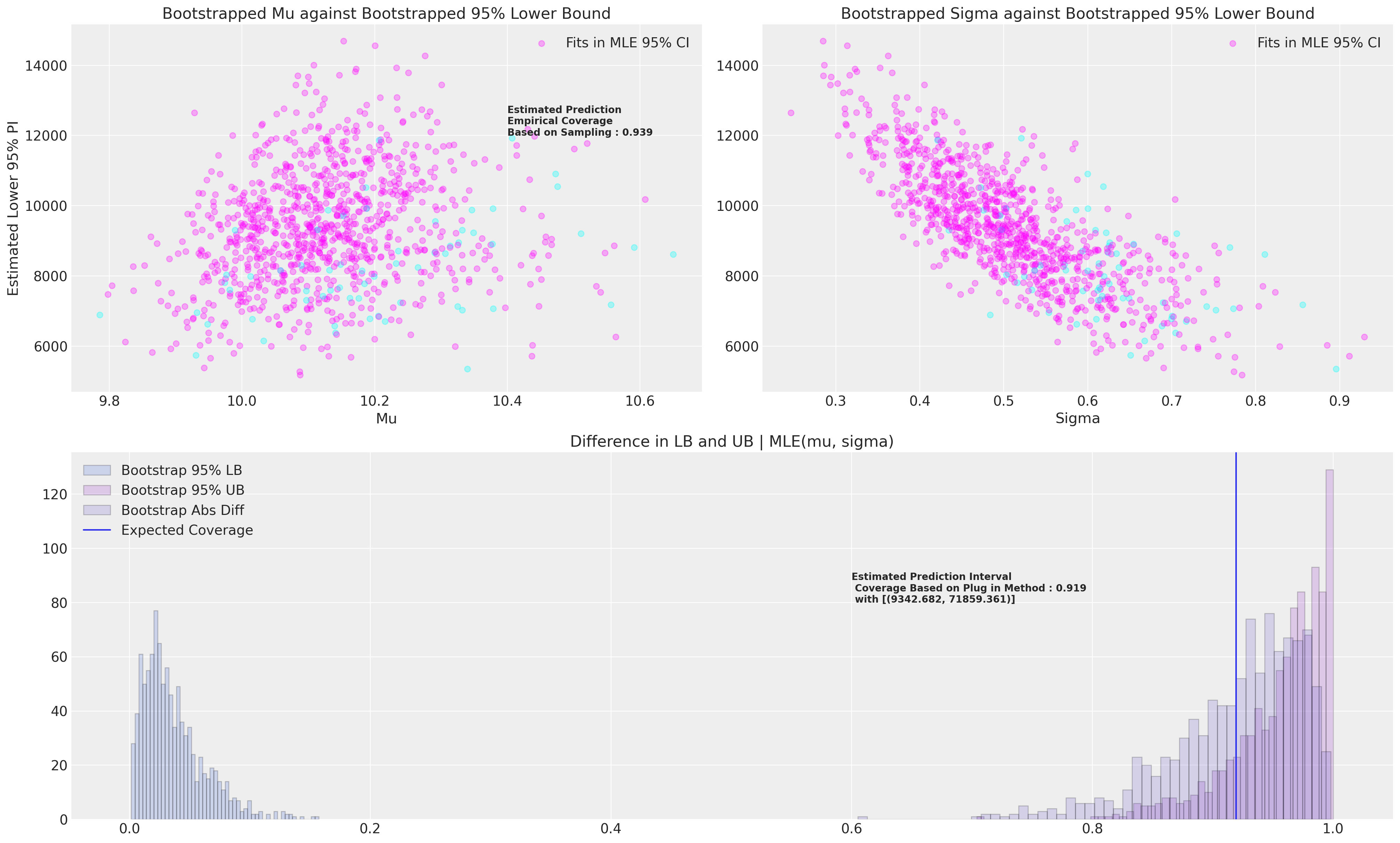
这些模拟应该比我们在这里进行的次数多得多。应该清楚地看到我们如何也可以改变MLE区间大小以达到所需的覆盖水平。
轴承座数据:贝叶斯可靠性分析研究#
接下来我们将研究一个参数拟合略微不那么干净的数据集。该数据最明显的特征是失败记录的数量较少。数据以周期格式记录,显示每个周期中风险 集的程度。
我们希望通过这个例子来展示如何在使用频率主义技术对减震器数据进行良好估计的情况下,增强对轴承座数据的处理。特别是我们将展示如何通过贝叶斯方法来解决出现的问题。
Show code cell source
bearing_cage_df = pd.read_csv(
    StringIO(
        """Hours,Censoring Indicator,Count
50,Censored,288
150,Censored,148
230,Failed,1
250,Censored,124
334,Failed,1
350,Censored,111
423,Failed,1
450,Censored,106
550,Censored,99
650,Censored,110
750,Censored,114
850,Censored,119
950,Censored,127
990,Failed,1
1009,Failed,1
1050,Censored,123
1150,Censored,93
1250,Censored,47
1350,Censored,41
1450,Censored,27
1510,Failed,1
1550,Censored,11
1650,Censored,6
1850,Censored,1
2050,Censored,2"""
    )
)


bearing_cage_df["t"] = bearing_cage_df["Hours"]
bearing_cage_df["failed"] = np.where(bearing_cage_df["Censoring Indicator"] == "Failed", 1, 0)
bearing_cage_df["censored"] = np.where(
    bearing_cage_df["Censoring Indicator"] == "Censored", bearing_cage_df["Count"], 0
)
bearing_cage_events = survival_table_from_events(
    bearing_cage_df["t"], bearing_cage_df["failed"], weights=bearing_cage_df["Count"]
).reset_index()
bearing_cage_events.rename(
    {"event_at": "t", "observed": "failed", "at_risk": "risk_set"}, axis=1, inplace=True
)
actuarial_table_bearings = make_actuarial_table(bearing_cage_events)

actuarial_table_bearings
| t | removed | failed | censored | entrance | risk_set | p_hat | 1-p_hat | S_hat | CH_hat | F_hat | V_hat | Standard_Error | CI_95_lb | CI_95_ub | ploting_position | logit_CI_95_lb | logit_CI_95_ub | |
|---|---|---|---|---|---|---|---|---|---|---|---|---|---|---|---|---|---|---|
| 0 | 0.0 | 0 | 0 | 0 | 1703 | 1703 | 0.000000 | 1.000000 | 1.000000 | -0.000000 | 0.000000 | 0.000000e+00 | 0.000000 | 0.0 | 0.000000 | 0.000000 | NaN | NaN |
| 1 | 50.0 | 288 | 0 | 288 | 0 | 1703 | 0.000000 | 1.000000 | 1.000000 | -0.000000 | 0.000000 | 0.000000e+00 | 0.000000 | 0.0 | 0.000000 | 0.000000 | NaN | NaN |
| 2 | 150.0 | 148 | 0 | 148 | 0 | 1415 | 0.000000 | 1.000000 | 1.000000 | -0.000000 | 0.000000 | 0.000000e+00 | 0.000000 | 0.0 | 0.000000 | 0.000000 | NaN | NaN |
| 3 | 230.0 | 1 | 1 | 0 | 0 | 1267 | 0.000789 | 0.999211 | 0.999211 | 0.000790 | 0.000789 | 6.224491e-07 | 0.000789 | 0.0 | 0.002336 | 0.000789 | 0.000111 | 0.005581 |
| 4 | 250.0 | 124 | 0 | 124 | 0 | 1266 | 0.000000 | 1.000000 | 0.999211 | 0.000790 | 0.000789 | 6.224491e-07 | 0.000789 | 0.0 | 0.002336 | 0.000789 | 0.000111 | 0.005581 |
| 5 | 334.0 | 1 | 1 | 0 | 0 | 1142 | 0.000876 | 0.999124 | 0.998336 | 0.001666 | 0.001664 | 1.386254e-06 | 0.001177 | 0.0 | 0.003972 | 0.001664 | 0.000415 | 0.006641 |
| 6 | 350.0 | 111 | 0 | 111 | 0 | 1141 | 0.000000 | 1.000000 | 0.998336 | 0.001666 | 0.001664 | 1.386254e-06 | 0.001177 | 0.0 | 0.003972 | 0.001664 | 0.000415 | 0.006641 |
| 7 | 423.0 | 1 | 1 | 0 | 0 | 1030 | 0.000971 | 0.999029 | 0.997367 | 0.002637 | 0.002633 | 2.322113e-06 | 0.001524 | 0.0 | 0.005620 | 0.002633 | 0.000846 | 0.008165 |
| 8 | 450.0 | 106 | 0 | 106 | 0 | 1029 | 0.000000 | 1.000000 | 0.997367 | 0.002637 | 0.002633 | 2.322113e-06 | 0.001524 | 0.0 | 0.005620 | 0.002633 | 0.000846 | 0.008165 |
| 9 | 550.0 | 99 | 0 | 99 | 0 | 923 | 0.000000 | 1.000000 | 0.997367 | 0.002637 | 0.002633 | 2.322113e-06 | 0.001524 | 0.0 | 0.005620 | 0.002633 | 0.000846 | 0.008165 |
| 10 | 650.0 | 110 | 0 | 110 | 0 | 824 | 0.000000 | 1.000000 | 0.997367 | 0.002637 | 0.002633 | 2.322113e-06 | 0.001524 | 0.0 | 0.005620 | 0.002633 | 0.000846 | 0.008165 |
| 11 | 750.0 | 114 | 0 | 114 | 0 | 714 | 0.000000 | 1.000000 | 0.997367 | 0.002637 | 0.002633 | 2.322113e-06 | 0.001524 | 0.0 | 0.005620 | 0.002633 | 0.000846 | 0.008165 |
| 12 | 850.0 | 119 | 0 | 119 | 0 | 600 | 0.000000 | 1.000000 | 0.997367 | 0.002637 | 0.002633 | 2.322113e-06 | 0.001524 | 0.0 | 0.005620 | 0.002633 | 0.000846 | 0.008165 |
| 13 | 950.0 | 127 | 0 | 127 | 0 | 481 | 0.000000 | 1.000000 | 0.997367 | 0.002637 | 0.002633 | 2.322113e-06 | 0.001524 | 0.0 | 0.005620 | 0.002633 | 0.000846 | 0.008165 |
| 14 | 990.0 | 1 | 1 | 0 | 0 | 354 | 0.002825 | 0.997175 | 0.994549 | 0.005466 | 0.005451 | 1.022444e-05 | 0.003198 | 0.0 | 0.011718 | 0.005451 | 0.001722 | 0.017117 |
| 15 | 1009.0 | 1 | 1 | 0 | 0 | 353 | 0.002833 | 0.997167 | 0.991732 | 0.008303 | 0.008268 | 1.808196e-05 | 0.004252 | 0.0 | 0.016603 | 0.008268 | 0.003008 | 0.022519 |
| 16 | 1050.0 | 123 | 0 | 123 | 0 | 352 | 0.000000 | 1.000000 | 0.991732 | 0.008303 | 0.008268 | 1.808196e-05 | 0.004252 | 0.0 | 0.016603 | 0.008268 | 0.003008 | 0.022519 |
| 17 | 1150.0 | 93 | 0 | 93 | 0 | 229 | 0.000000 | 1.000000 | 0.991732 | 0.008303 | 0.008268 | 1.808196e-05 | 0.004252 | 0.0 | 0.016603 | 0.008268 | 0.003008 | 0.022519 |
| 18 | 1250.0 | 47 | 0 | 47 | 0 | 136 | 0.000000 | 1.000000 | 0.991732 | 0.008303 | 0.008268 | 1.808196e-05 | 0.004252 | 0.0 | 0.016603 | 0.008268 | 0.003008 | 0.022519 |
| 19 | 1350.0 | 41 | 0 | 41 | 0 | 89 | 0.000000 | 1.000000 | 0.991732 | 0.008303 | 0.008268 | 1.808196e-05 | 0.004252 | 0.0 | 0.016603 | 0.008268 | 0.003008 | 0.022519 |
| 20 | 1450.0 | 27 | 0 | 27 | 0 | 48 | 0.000000 | 1.000000 | 0.991732 | 0.008303 | 0.008268 | 1.808196e-05 | 0.004252 | 0.0 | 0.016603 | 0.008268 | 0.003008 | 0.022519 |
| 21 | 1510.0 | 1 | 1 | 0 | 0 | 21 | 0.047619 | 0.952381 | 0.944506 | 0.057093 | 0.055494 | 2.140430e-03 | 0.046265 | 0.0 | 0.146173 | 0.055494 | 0.010308 | 0.248927 |
| 22 | 1550.0 | 11 | 0 | 11 | 0 | 20 | 0.000000 | 1.000000 | 0.944506 | 0.057093 | 0.055494 | 2.140430e-03 | 0.046265 | 0.0 | 0.146173 | 0.055494 | 0.010308 | 0.248927 |
| 23 | 1650.0 | 6 | 0 | 6 | 0 | 9 | 0.000000 | 1.000000 | 0.944506 | 0.057093 | 0.055494 | 2.140430e-03 | 0.046265 | 0.0 | 0.146173 | 0.055494 | 0.010308 | 0.248927 |
| 24 | 1850.0 | 1 | 0 | 1 | 0 | 3 | 0.000000 | 1.000000 | 0.944506 | 0.057093 | 0.055494 | 2.140430e-03 | 0.046265 | 0.0 | 0.146173 | 0.055494 | 0.010308 | 0.248927 |
| 25 | 2050.0 | 2 | 0 | 2 | 0 | 2 | 0.000000 | 1.000000 | 0.944506 | 0.057093 | 0.055494 | 2.140430e-03 | 0.046265 | 0.0 | 0.146173 | 0.055494 | 0.010308 | 0.248927 |
为了估计单变量或非参数的CDF,我们需要将周期格式的数据分解为项目-周期格式。
项目周期数据格式#
item_period = bearing_cage_df["Hours"].to_list() * bearing_cage_df["Count"].sum()
ids = [[i] * 25 for i in range(bearing_cage_df["Count"].sum())]
ids = [int(i) for l in ids for i in l]
item_period_bearing_cage = pd.DataFrame(item_period, columns=["t"])
item_period_bearing_cage["id"] = ids
item_period_bearing_cage["failed"] = np.zeros(len(item_period_bearing_cage))

## Censor appropriate number of ids
unique_ids = item_period_bearing_cage["id"].unique()
censored = bearing_cage_df[bearing_cage_df["Censoring Indicator"] == "Censored"]
i = 0
stack = []
for hour, count, idx in zip(censored["Hours"], censored["Count"], censored["Count"].cumsum()):
    temp = item_period_bearing_cage[
        item_period_bearing_cage["id"].isin(unique_ids[i:idx])
        & (item_period_bearing_cage["t"] == hour)
    ]
    stack.append(temp)
    i = idx

censored_clean = pd.concat(stack)

### Add  appropriate number of failings
stack = []
unique_times = censored_clean["t"].unique()
for id, fail_time in zip(
    [9999, 9998, 9997, 9996, 9995, 9994],
    bearing_cage_df[bearing_cage_df["failed"] == 1]["t"].values,
):
    temp = pd.DataFrame(unique_times[unique_times < fail_time], columns=["t"])
    temp["id"] = id
    temp["failed"] = 0
    temp = pd.concat([temp, pd.DataFrame({"t": [fail_time], "id": [id], "failed": [1]}, index=[0])])
    stack.append(temp)

failed_clean = pd.concat(stack).sort_values(["id", "t"])
censored_clean
item_period_bearing_cage = pd.concat([failed_clean, censored_clean])
## Transpose for more concise visual
item_period_bearing_cage.head(30).T
| 0 | 1 | 2 | 3 | 4 | 5 | 6 | 7 | 8 | 9 | ... | 4 | 5 | 6 | 7 | 8 | 9 | 0 | 0 | 1 | 2 | |
|---|---|---|---|---|---|---|---|---|---|---|---|---|---|---|---|---|---|---|---|---|---|
| t | 50.0 | 150.0 | 250.0 | 350.0 | 450.0 | 550.0 | 650.0 | 750.0 | 850.0 | 950.0 | ... | 450.0 | 550.0 | 650.0 | 750.0 | 850.0 | 950.0 | 1009.0 | 50.0 | 150.0 | 250.0 |
| id | 9994.0 | 9994.0 | 9994.0 | 9994.0 | 9994.0 | 9994.0 | 9994.0 | 9994.0 | 9994.0 | 9994.0 | ... | 9995.0 | 9995.0 | 9995.0 | 9995.0 | 9995.0 | 9995.0 | 9995.0 | 9996.0 | 9996.0 | 9996.0 |
| failed | 0.0 | 0.0 | 0.0 | 0.0 | 0.0 | 0.0 | 0.0 | 0.0 | 0.0 | 0.0 | ... | 0.0 | 0.0 | 0.0 | 0.0 | 0.0 | 0.0 | 1.0 | 0.0 | 0.0 | 0.0 |
3行 × 30列
assert item_period_bearing_cage["id"].nunique() == 1703
assert item_period_bearing_cage["failed"].sum() == 6
assert item_period_bearing_cage[item_period_bearing_cage["t"] >= 1850]["id"].nunique() == 3
当我们绘制经验累积分布函数时,我们看到y轴的最大高度仅为0.05。一个简单的最大似然估计拟合在数据观测范围之外的外推中会严重出错。
ax = plot_cdfs(
    actuarial_table_bearings,
    title="Bearings",
    dist_fits=False,
    xy=(20, 0.7),
    item_period=item_period_bearing_cage,
)
概率图:在受限线性范围内比较CDF#
在本节中,我们将使用线性化MLE拟合的技术,以便能够进行视觉上的“拟合优度”检查。这些类型的图依赖于一种转换,该转换可以应用于位置和尺度分布,将它们的CDF转换为线性空间。
对于对数正态分布和威布尔分布的拟合,我们可以在线性空间中表示它们的CDF,作为对数值t与适当的\(CDF^{-1}\)之间的关系。
Show code cell source
def sev_ppf(p):
    return np.log(-np.log(1 - p))


mosaic = """AABB
            CCCC"""
fig, axs = plt.subplot_mosaic(mosaic=mosaic, figsize=(20, 15))
axs = [axs[k] for k in axs.keys()]
ax = axs[0]
ax2 = axs[1]
ax3 = axs[2]
ax.plot(
    np.log(actuarial_table_bearings["t"]),
    norm.ppf(actuarial_table_bearings["logit_CI_95_ub"]),
    "-o",
    label="Non-Parametric CI UB",
    color="slateblue",
)
ax.scatter(
    np.log(actuarial_table_bearings["t"]),
    norm.ppf(actuarial_table_bearings["ploting_position"]),
    label="Non-Parametric CDF",
    color="black",
)
ax.plot(
    np.log(actuarial_table_bearings["t"]),
    norm.ppf(actuarial_table_bearings["logit_CI_95_lb"]),
    "-o",
    label="Non-Parametric CI LB",
    color="slateblue",
)
for mu in np.linspace(10, 12, 3):
    for sigma in np.linspace(1.6, 1.9, 3):
        rv = lognorm(s=sigma, scale=np.exp(mu))
        ax.plot(
            np.log(actuarial_table_bearings["t"]),
            norm.ppf(rv.cdf(actuarial_table_bearings["t"])),
            "--",
            label=f"LN({np.round(mu, 3)}, {np.round(sigma, 3)})",
            color="grey",
        )

lnf = LogNormalFitter().fit(item_period_bearing_cage["t"], item_period_bearing_cage["failed"])
rv = lognorm(s=lnf.sigma_, scale=np.exp(lnf.mu_))
ax.plot(
    np.log(actuarial_table_bearings["t"]),
    norm.ppf(rv.cdf(actuarial_table_bearings["t"])),
    "--",
    label=f"MLE LN({np.round(lnf.mu_, 3)}, {np.round(lnf.sigma_, 3)})",
    color="RED",
)

for r in np.linspace(1, 2, 3):
    for s in np.linspace(12000, 25000, 2):
        rv = weibull_min(c=r, scale=s)
        ax2.plot(
            np.log(actuarial_table_bearings["t"]),
            sev_ppf(rv.cdf(actuarial_table_bearings["t"])),
            "--",
            label=f"Wb({np.round(s, 3)}, {np.round(r, 3)})",
            color="lightblue",
        )


wbf = WeibullFitter().fit(item_period_bearing_cage["t"], item_period_bearing_cage["failed"])
rv = weibull_min(c=wbf.rho_, scale=wbf.lambda_)
ax2.plot(
    np.log(actuarial_table_bearings["t"]),
    sev_ppf(rv.cdf(actuarial_table_bearings["t"])),
    "--",
    label=f"MLE Wb({np.round(wbf.lambda_, 3)}, {np.round(wbf.rho_, 3)})",
    color="red",
)

ax2.plot(
    np.log(actuarial_table_bearings["t"]),
    sev_ppf(actuarial_table_bearings["logit_CI_95_ub"]),
    "-o",
    label="Non-Parametric CI UB",
    color="slateblue",
)
ax2.scatter(
    np.log(actuarial_table_bearings["t"]),
    sev_ppf(actuarial_table_bearings["ploting_position"]),
    label="Non-Parametric CDF",
    color="black",
)
ax2.plot(
    np.log(actuarial_table_bearings["t"]),
    sev_ppf(actuarial_table_bearings["logit_CI_95_lb"]),
    "-o",
    label="Non-Parametric CI LB",
    color="slateblue",
)

ax3.plot(
    actuarial_table_bearings["t"],
    actuarial_table_bearings["logit_CI_95_ub"],
    "-o",
    label="Non-Parametric CI UB",
    color="slateblue",
)
ax3.scatter(
    actuarial_table_bearings["t"],
    actuarial_table_bearings["F_hat"],
    label="Non-Parametric CDF",
    color="black",
)
ax3.plot(
    actuarial_table_bearings["t"],
    actuarial_table_bearings["logit_CI_95_lb"],
    "-o",
    label="Non-Parametric CI LB",
    color="slateblue",
)
lnf.plot_cumulative_density(ax=ax3, color="cyan")
wbf.plot_cumulative_density(ax=ax3, color="darkorchid")


ax2.set_title("Linearizing the Weibull CDF", fontsize=20)
ax.set_title("Linearizing the Lognormal CDF", fontsize=20)
ax3.set_title("MLE CDF Fits", fontsize=20)
ax.legend()
ax.set_xlabel("Time")
ax2.set_xlabel("Time")
xticks = np.round(np.linspace(0, actuarial_table_bearings["t"].max(), 10), 1)
yticks = np.round(np.linspace(0, actuarial_table_bearings["F_hat"].max(), 10), 4)
ax.set_xticklabels(xticks)
ax.set_yticklabels(yticks)
ax2.set_xticklabels(xticks)
ax2.set_yticklabels([])
ax2.legend()
ax.set_ylabel("Fraction Failing");
/home/oriol/bin/miniconda3/envs/releases/lib/python3.10/site-packages/pandas/core/arraylike.py:402: RuntimeWarning: divide by zero encountered in log
  result = getattr(ufunc, method)(*inputs, **kwargs)
/home/oriol/bin/miniconda3/envs/releases/lib/python3.10/site-packages/pandas/core/arraylike.py:402: RuntimeWarning: divide by zero encountered in log
  result = getattr(ufunc, method)(*inputs, **kwargs)
/tmp/ipykernel_29435/2628457585.py:2: RuntimeWarning: divide by zero encountered in log
  return np.log(-np.log(1 - p))
/tmp/ipykernel_29435/2628457585.py:128: UserWarning: FixedFormatter should only be used together with FixedLocator
  ax.set_xticklabels(xticks)
/tmp/ipykernel_29435/2628457585.py:129: UserWarning: FixedFormatter should only be used together with FixedLocator
  ax.set_yticklabels(yticks)
/tmp/ipykernel_29435/2628457585.py:130: UserWarning: FixedFormatter should only be used together with FixedLocator
  ax2.set_xticklabels(xticks)
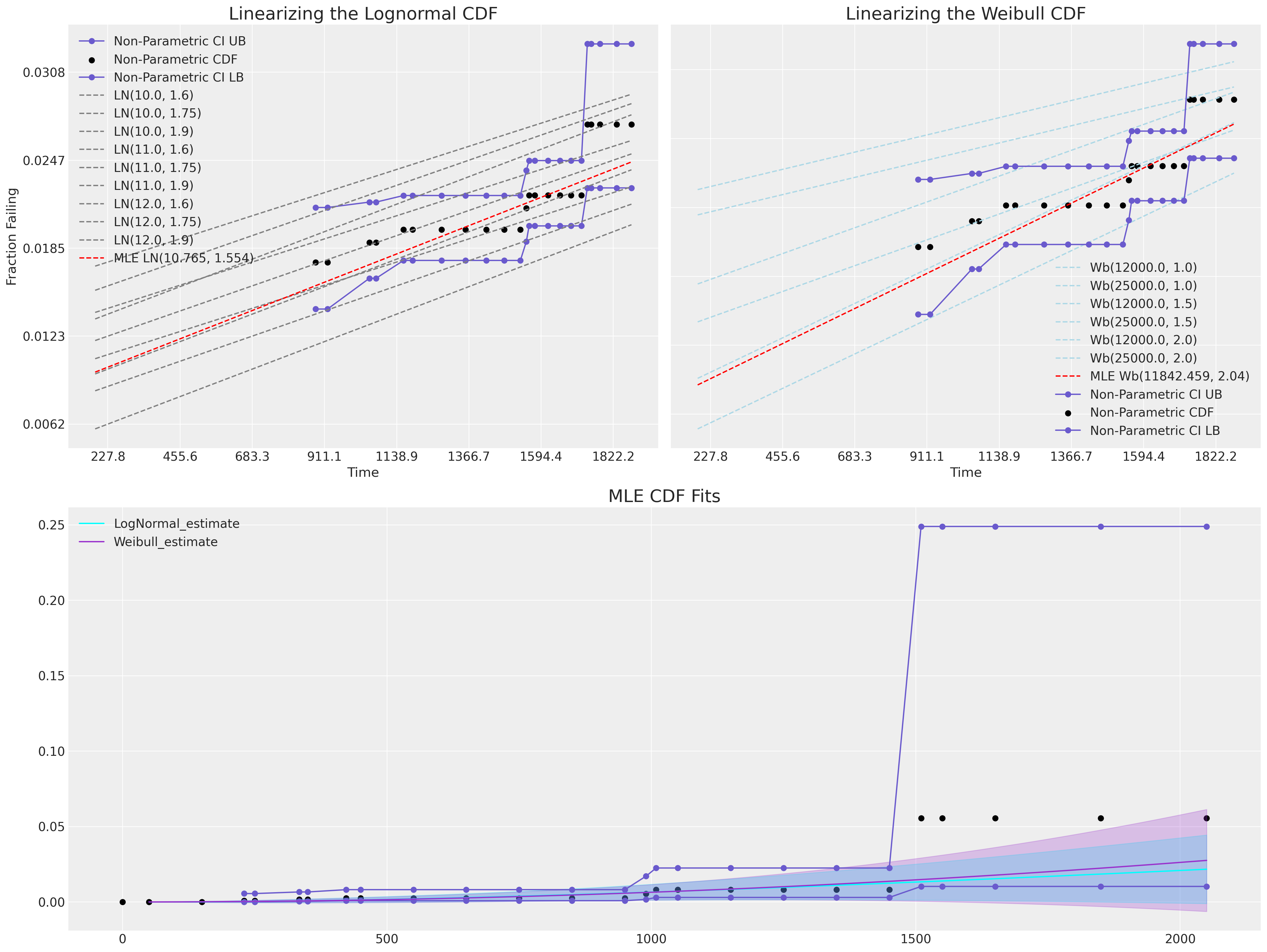
我们可以看到,这里无论是MLE拟合都无法覆盖观测数据的范围。
可靠性数据的贝叶斯建模#
我们现在已经了解了如何使用频率主义或最大似然估计框架对稀疏可靠性进行参数模型拟合的建模和可视化。我们希望现在展示如何在贝叶斯范式中实现相同风格的推断。
与MLE范式一样,我们需要对删失似然进行建模。对于我们上面看到的大多数对数位置分布,似然性表示为分布pdf \(\phi\) 和cdf \(\Phi\) 的组合的函数,具体应用取决于数据点是否在时间窗口内完全观察到或被删失。
其中 \(\delta_{i}\) 是指示观测值是失败还是右删失观测值的指标。根据删失观测值的性质,可以通过对CDF进行类似的修改来包括更复杂的删失类型。
直接使用PYMC实现Weibull生存分析#
我们使用两种不同的先验规范拟合了该模型的两个版本,一种采用数据上的模糊均匀先验,另一种则指定了更接近最大似然估计(MLE)拟合的先验。我们将在下面展示先验规范对模型与观测数据校准的影响。
def weibull_lccdf(y, alpha, beta):
    """Log complementary cdf of Weibull distribution."""
    return -((y / beta) ** alpha)


item_period_max = item_period_bearing_cage.groupby("id")[["t", "failed"]].max()
y = item_period_max["t"].values
censored = ~item_period_max["failed"].values.astype(bool)


priors = {"beta": [100, 15_000], "alpha": [4, 1, 0.02, 8]}
priors_informative = {"beta": [10_000, 500], "alpha": [2, 0.5, 0.02, 3]}


def make_model(p, info=False):
    with pm.Model() as model:
        if info:
            beta = pm.Normal("beta", p["beta"][0], p["beta"][1])
        else:
            beta = pm.Uniform("beta", p["beta"][0], p["beta"][1])
        alpha = pm.TruncatedNormal(
            "alpha", p["alpha"][0], p["alpha"][1], lower=p["alpha"][2], upper=p["alpha"][3]
        )

        y_obs = pm.Weibull("y_obs", alpha=alpha, beta=beta, observed=y[~censored])
        y_cens = pm.Potential("y_cens", weibull_lccdf(y[censored], alpha, beta))
        idata = pm.sample_prior_predictive()
        idata.extend(pm.sample(random_seed=100, target_accept=0.95))
        idata.extend(pm.sample_posterior_predictive(idata))

    return idata, model


idata, model = make_model(priors)
idata_informative, model = make_model(priors_informative, info=True)
/tmp/ipykernel_29435/305144286.py:28: UserWarning: The effect of Potentials on other parameters is ignored during prior predictive sampling. This is likely to lead to invalid or biased predictive samples.
  idata = pm.sample_prior_predictive()
Sampling: [alpha, beta, y_obs]
Auto-assigning NUTS sampler...
Initializing NUTS using jitter+adapt_diag...
Multiprocess sampling (4 chains in 4 jobs)
NUTS: [beta, alpha]
Sampling 4 chains for 1_000 tune and 1_000 draw iterations (4_000 + 4_000 draws total) took 6 seconds.
/tmp/ipykernel_29435/305144286.py:30: UserWarning: The effect of Potentials on other parameters is ignored during posterior predictive sampling. This is likely to lead to invalid or biased predictive samples.
  idata.extend(pm.sample_posterior_predictive(idata))
Sampling: [y_obs]
idata
-
<xarray.Dataset> Dimensions: (chain: 4, draw: 1000) Coordinates: * chain (chain) int64 0 1 2 3 * draw (draw) int64 0 1 2 3 4 5 6 7 8 ... 992 993 994 995 996 997 998 999 Data variables: beta (chain, draw) float64 7.427e+03 8.514e+03 ... 1.013e+04 5.044e+03 alpha (chain, draw) float64 2.232 2.385 2.49 2.55 ... 2.437 2.503 2.898 Attributes: created_at: 2023-01-15T20:06:41.169437 arviz_version: 0.13.0 inference_library: pymc inference_library_version: 5.0.0 sampling_time: 6.423727989196777 tuning_steps: 1000 -
<xarray.Dataset> Dimensions: (chain: 4, draw: 1000, y_obs_dim_2: 6) Coordinates: * chain (chain) int64 0 1 2 3 * draw (draw) int64 0 1 2 3 4 5 6 7 ... 993 994 995 996 997 998 999 * y_obs_dim_2 (y_obs_dim_2) int64 0 1 2 3 4 5 Data variables: y_obs (chain, draw, y_obs_dim_2) float64 6.406e+03 ... 5.59e+03 Attributes: created_at: 2023-01-15T20:06:42.789072 arviz_version: 0.13.0 inference_library: pymc inference_library_version: 5.0.0 -
<xarray.Dataset> Dimensions: (chain: 4, draw: 1000) Coordinates: * chain (chain) int64 0 1 2 3 * draw (draw) int64 0 1 2 3 4 5 ... 994 995 996 997 998 999 Data variables: (12/17) perf_counter_diff (chain, draw) float64 0.0008238 ... 0.002601 n_steps (chain, draw) float64 3.0 3.0 7.0 ... 11.0 7.0 9.0 acceptance_rate (chain, draw) float64 0.9404 1.0 ... 0.9876 0.9424 smallest_eigval (chain, draw) float64 nan nan nan nan ... nan nan nan largest_eigval (chain, draw) float64 nan nan nan nan ... nan nan nan lp (chain, draw) float64 -80.96 -79.7 ... -81.05 -79.99 ... ... step_size_bar (chain, draw) float64 0.1791 0.1791 ... 0.1591 0.1591 reached_max_treedepth (chain, draw) bool False False False ... False False diverging (chain, draw) bool False False False ... False False process_time_diff (chain, draw) float64 0.0008239 ... 0.002601 index_in_trajectory (chain, draw) int64 -2 2 -3 -2 2 -2 ... -2 -1 -3 1 -6 perf_counter_start (chain, draw) float64 1.153e+04 ... 1.153e+04 Attributes: created_at: 2023-01-15T20:06:41.180463 arviz_version: 0.13.0 inference_library: pymc inference_library_version: 5.0.0 sampling_time: 6.423727989196777 tuning_steps: 1000 -
<xarray.Dataset> Dimensions: (chain: 1, draw: 500) Coordinates: * chain (chain) int64 0 * draw (draw) int64 0 1 2 3 4 5 6 7 8 ... 492 493 494 495 496 497 498 499 Data variables: alpha (chain, draw) float64 3.896 5.607 4.329 5.377 ... 3.828 4.875 3.723 beta (chain, draw) float64 6.915e+03 1.293e+04 ... 6.599e+03 1.244e+04 Attributes: created_at: 2023-01-15T20:06:29.497052 arviz_version: 0.13.0 inference_library: pymc inference_library_version: 5.0.0 -
<xarray.Dataset> Dimensions: (chain: 1, draw: 500, y_obs_dim_0: 6) Coordinates: * chain (chain) int64 0 * draw (draw) int64 0 1 2 3 4 5 6 7 ... 493 494 495 496 497 498 499 * y_obs_dim_0 (y_obs_dim_0) int64 0 1 2 3 4 5 Data variables: y_obs (chain, draw, y_obs_dim_0) float64 6.422e+03 ... 1.476e+04 Attributes: created_at: 2023-01-15T20:06:29.500007 arviz_version: 0.13.0 inference_library: pymc inference_library_version: 5.0.0 -
<xarray.Dataset>
Dimensions:      (y_obs_dim_0: 6)
Coordinates:
  * y_obs_dim_0  (y_obs_dim_0) int64 0 1 2 3 4 5
Data variables:
    y_obs        (y_obs_dim_0) float64 1.51e+03 1.009e+03 990.0 ... 334.0 230.0
Attributes:
    created_at:                 2023-01-15T20:06:29.501343
    arviz_version:              0.13.0
    inference_library:          pymc
    inference_library_version:  5.0.0
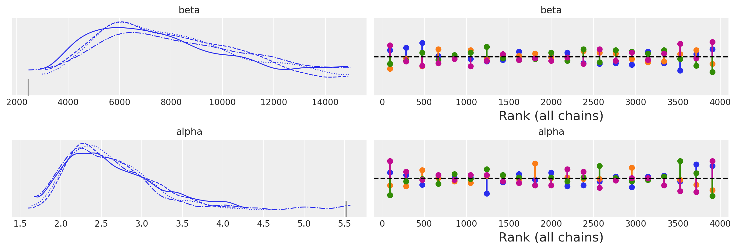
az.plot_trace(idata, kind="rank_vlines");
az.plot_trace(idata_informative, kind="rank_vlines");
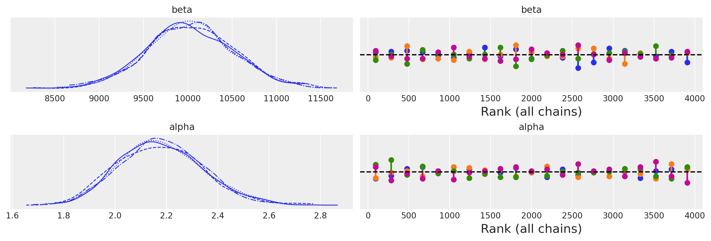
az.summary(idata)
| mean | sd | hdi_3% | hdi_97% | mcse_mean | mcse_sd | ess_bulk | ess_tail | r_hat | |
|---|---|---|---|---|---|---|---|---|---|
| beta | 8149.835 | 2916.378 | 3479.929 | 13787.447 | 111.293 | 78.729 | 612.0 | 371.0 | 1.01 |
| alpha | 2.626 | 0.558 | 1.779 | 3.631 | 0.030 | 0.025 | 616.0 | 353.0 | 1.01 |
az.summary(idata_informative)
| mean | sd | hdi_3% | hdi_97% | mcse_mean | mcse_sd | ess_bulk | ess_tail | r_hat | |
|---|---|---|---|---|---|---|---|---|---|
| beta | 10031.200 | 491.768 | 9110.601 | 10975.705 | 10.891 | 7.742 | 2045.0 | 1940.0 | 1.0 |
| alpha | 2.181 | 0.166 | 1.875 | 2.487 | 0.004 | 0.003 | 2240.0 | 1758.0 | 1.0 |
joint_draws = az.extract(idata, num_samples=1000)[["alpha", "beta"]]
alphas = joint_draws["alpha"].values
betas = joint_draws["beta"].values

joint_draws_informative = az.extract(idata_informative, num_samples=1000)[["alpha", "beta"]]
alphas_informative = joint_draws_informative["alpha"].values
betas_informative = joint_draws_informative["beta"].values

mosaic = """AAAA
            BBCC"""
fig, axs = plt.subplot_mosaic(mosaic=mosaic, figsize=(20, 13))
axs = [axs[k] for k in axs.keys()]
ax = axs[0]
ax1 = axs[2]
ax2 = axs[1]
hist_data = []
for i in range(1000):
    draws = pm.draw(pm.Weibull.dist(alpha=alphas[i], beta=betas[i]), 1000)
    qe, pe = ecdf(draws)
    lkup = dict(zip(pe, qe))
    hist_data.append([lkup[0.1], lkup[0.05]])
    ax.plot(qe, pe, color="slateblue", alpha=0.1)
hist_data_info = []
for i in range(1000):
    draws = pm.draw(pm.Weibull.dist(alpha=alphas_informative[i], beta=betas_informative[i]), 1000)
    qe, pe = ecdf(draws)
    lkup = dict(zip(pe, qe))
    hist_data_info.append([lkup[0.1], lkup[0.05]])
    ax.plot(qe, pe, color="pink", alpha=0.1)
hist_data = pd.DataFrame(hist_data, columns=["p10", "p05"])
hist_data_info = pd.DataFrame(hist_data_info, columns=["p10", "p05"])
draws = pm.draw(pm.Weibull.dist(alpha=np.mean(alphas), beta=np.mean(betas)), 1000)
qe, pe = ecdf(draws)
ax.plot(qe, pe, color="purple", label="Expected CDF Uninformative Prior")
draws = pm.draw(
    pm.Weibull.dist(alpha=np.mean(alphas_informative), beta=np.mean(betas_informative)), 1000
)
qe, pe = ecdf(draws)
ax.plot(qe, pe, color="magenta", label="Expected CDF Informative Prior")
ax.plot(
    actuarial_table_bearings["t"],
    actuarial_table_bearings["logit_CI_95_ub"],
    "--",
    label="Non-Parametric CI UB",
    color="black",
)
ax.plot(
    actuarial_table_bearings["t"],
    actuarial_table_bearings["F_hat"],
    "-o",
    label="Non-Parametric CDF",
    color="black",
    alpha=1,
)
ax.plot(
    actuarial_table_bearings["t"],
    actuarial_table_bearings["logit_CI_95_lb"],
    "--",
    label="Non-Parametric CI LB",
    color="black",
)
ax.set_xlim(0, 2500)
ax.set_title(
    "Bayesian Estimation of Uncertainty in the Posterior Predictive CDF \n Informative and Non-Informative Priors",
    fontsize=20,
)
ax.set_ylabel("Fraction Failing")
ax.set_xlabel("Time")
ax1.hist(
    hist_data["p10"], bins=30, ec="black", color="skyblue", alpha=0.4, label="Uninformative Prior"
)
ax1.hist(
    hist_data_info["p10"],
    bins=30,
    ec="black",
    color="slateblue",
    alpha=0.4,
    label="Informative Prior",
)
ax1.set_title("Distribution of 10% failure Time", fontsize=20)
ax1.legend()
ax2.hist(
    hist_data["p05"], bins=30, ec="black", color="cyan", alpha=0.4, label="Uninformative Prior"
)
ax2.hist(
    hist_data_info["p05"], bins=30, ec="black", color="pink", alpha=0.4, label="Informative Prior"
)
ax2.legend()
ax2.set_title("Distribution of 5% failure Time", fontsize=20)
wbf = WeibullFitter().fit(item_period_bearing_cage["t"] + 1e-25, item_period_bearing_cage["failed"])
wbf.plot_cumulative_density(ax=ax, color="cyan", label="Weibull MLE Fit")
ax.legend()
ax.set_ylim(0, 0.25);
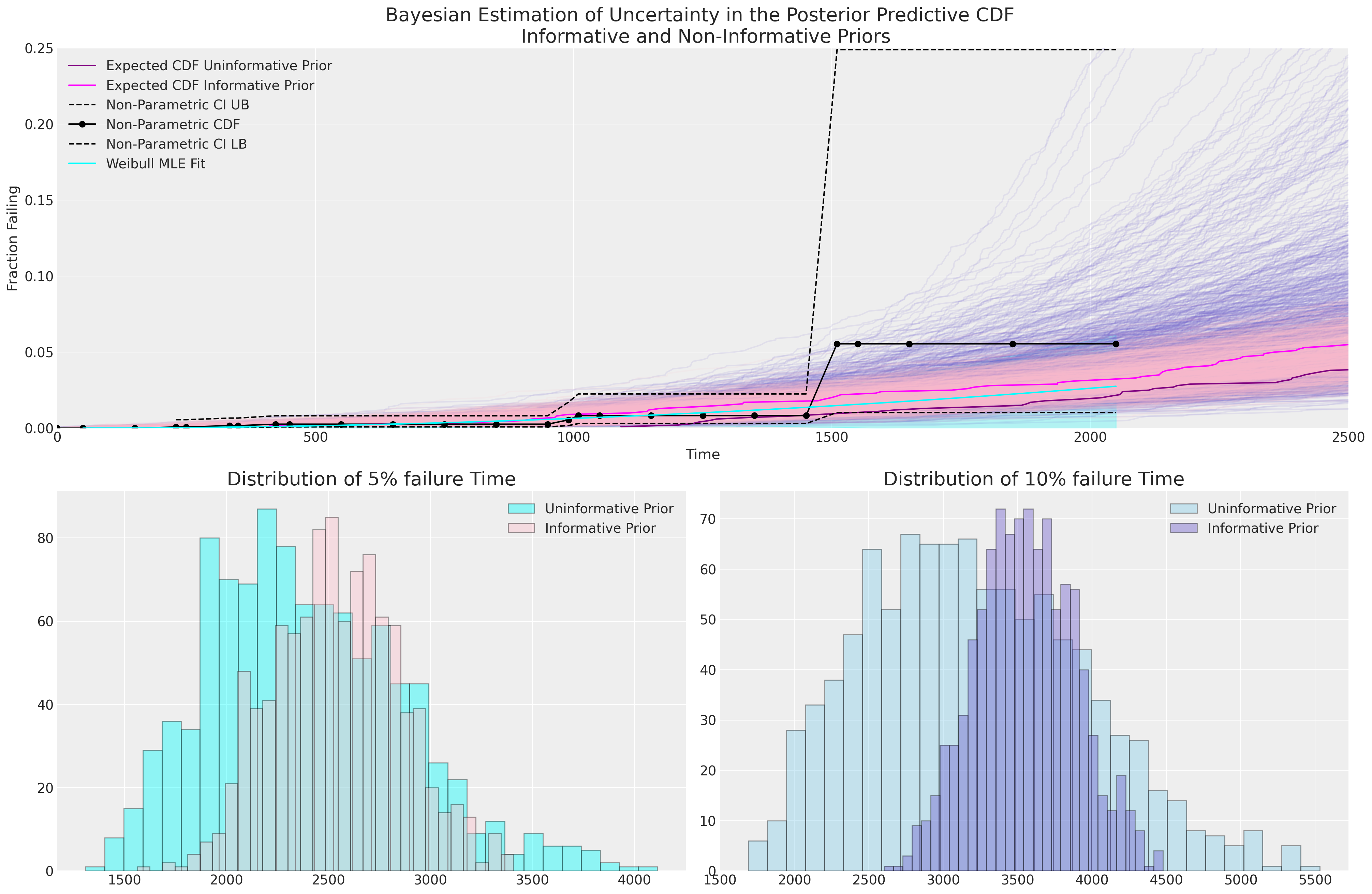
我们可以看到,由我们故意模糊的先验驱动的贝叶斯不确定性估计比我们的MLE拟合和无信息先验包含了更多的不确定性,并且无信息先验意味着5%和10%失效时间的预测分布更宽。使用无信息先验的贝叶斯模型似乎更好地捕捉了我们CDF的非参数估计中的不确定性,但没有更多信息,很难判断哪个模型更合适。
在数据稀疏的情况下,每个模型拟合的失败百分比随时间变化的实际估计尤为关键。这是一个有意义的检查,我们可以与主题专家讨论他们对产品10%失败时间的期望和范围的合理性。
预测区间内的失败次数#
由于我们观察到的故障数据极其稀疏,我们必须非常小心地外推超出观察到的时间范围,但我们可以询问在我们的累积分布函数(cdf)的较低尾部可预测的故障数量。这提供了另一种观察数据的视角,有助于与主题专家进行讨论。
插件估计#
假设我们想知道在150到600小时的服务时间内会有多少轴承失效。我们可以根据估计的CDF和未来新轴承的数量来计算。我们首先计算:
为区间内发生的故障建立概率,然后区间内故障数量的点预测由 risk_set*\(\hat{\rho}\) 给出。
mle_fit = weibull_min(c=2, scale=10_000)
rho = mle_fit.cdf(600) - mle_fit.cdf(150) / (1 - mle_fit.cdf(150))
print("Rho:", rho)
print("N at Risk:", 1700)
print("Expected Number Failing in between 150 and 600 hours:", 1700 * rho)
print("Lower Bound 95% PI :", binom(1700, rho).ppf(0.05))
print("Upper Bound 95% PI:", binom(1700, rho).ppf(0.95))
Rho: 0.0033685024546080927
N at Risk: 1700
Expected Number Failing in between 150 and 600 hours: 5.7264541728337575
Lower Bound 95% PI : 2.0
Upper Bound 95% PI: 10.0
在贝叶斯后验上应用相同的过程#
我们将使用无信息模型的后验预测分布。这里我们展示了如何推导出时间间隔内故障数量的95%预测区间估计中的不确定性。正如我们上面所看到的,这个过程的MLE替代方法是基于bootstrap采样生成预测分布。bootstrap过程往往与使用MLE估计的插件过程一致,并且缺乏指定先验信息的灵活性。
import xarray as xr

from xarray_einstats.stats import XrContinuousRV, XrDiscreteRV


def PI_failures(joint_draws, lp, up, n_at_risk):
    fit = XrContinuousRV(weibull_min, joint_draws["alpha"], scale=joint_draws["beta"])
    rho = fit.cdf(up) - fit.cdf(lp) / (1 - fit.cdf(lp))
    lub = XrDiscreteRV(binom, n_at_risk, rho).ppf([0.05, 0.95])
    lb, ub = lub.sel(quantile=0.05, drop=True), lub.sel(quantile=0.95, drop=True)
    point_prediction = n_at_risk * rho
    return xr.Dataset(
        {"rho": rho, "n_at_risk": n_at_risk, "lb": lb, "ub": ub, "expected": point_prediction}
    )


output_ds = PI_failures(joint_draws, 150, 600, 1700)
output_ds
<xarray.Dataset>
Dimensions:    (sample: 1000)
Coordinates:
  * sample     (sample) object MultiIndex
  * chain      (sample) int64 1 0 0 0 2 1 1 2 1 3 0 2 ... 1 3 2 3 0 1 3 3 0 1 2
  * draw       (sample) int64 776 334 531 469 19 675 ... 437 470 242 662 316 63
Data variables:
    rho        (sample) float64 0.0007735 0.004392 ... 0.001465 0.001462
    n_at_risk  int64 1700
    lb         (sample) float64 0.0 3.0 0.0 0.0 0.0 1.0 ... 0.0 1.0 0.0 0.0 0.0
    ub         (sample) float64 3.0 12.0 5.0 5.0 4.0 7.0 ... 5.0 7.0 6.0 5.0 5.0
expected (sample) float64 1.315 7.466 2.24 2.518 ... 2.835 2.491 2.486def cost_func(failures, power):
### Imagined cost function for failing item e.g. refunds required
return np.power(failures, power)
mosaic = """AAAA
BBCC"""
fig, axs = plt.subplot_mosaic(mosaic=mosaic, figsize=(20, 12))
axs = [axs[k] for k in axs.keys()]
ax = axs[0]
ax1 = axs[1]
ax2 = axs[2]
ax.scatter(
joint_draws["alpha"],
output_ds["expected"],
c=joint_draws["beta"],
cmap=cm.cool,
alpha=0.3,
label="Coloured by function of Beta values",
)
ax.legend()
ax.set_ylabel("Expected Failures")
ax.set_xlabel("Alpha")
ax.set_title(
"Posterior Predictive Expected Failure Count between 150-600 hours \nas a function of Weibull(alpha, beta)",
fontsize=20,
)
ax1.hist(
output_ds["lb"],
ec="black",
color="slateblue",
label="95% PI Lower Bound on Failure Count",
alpha=0.3,
)
ax1.axvline(output_ds["lb"].mean(), label="Expected 95% PI Lower Bound on Failure Count")
ax1.axvline(output_ds["ub"].mean(), label="Expected 95% PI Upper Bound on Failure Count")
ax1.hist(
output_ds["ub"],
ec="black",
color="cyan",
label="95% PI Upper Bound on Failure Count",
bins=20,
alpha=0.3,
)
ax1.hist(
output_ds["expected"], ec="black", color="pink", label="Expected Count of Failures", bins=20
)
ax1.set_title("Uncertainty in the Posterior Prediction Interval of Failure Counts", fontsize=20)
ax1.legend()
ax2.set_title("Expected Costs Distribution(s) \nbased on implied Failure counts", fontsize=20)
ax2.hist(
cost_func(output_ds["expected"], 2.3),
label="Cost(failures,2)",
color="royalblue",
alpha=0.3,
ec="black",
bins=20,
)
ax2.hist(
cost_func(output_ds["expected"], 2),
label="Cost(failures,2.3)",
color="red",
alpha=0.5,
ec="black",
bins=20,
)
ax2.set_xlabel("$ cost")
# ax2.set_xlim(-60, 0)
ax2.legend();
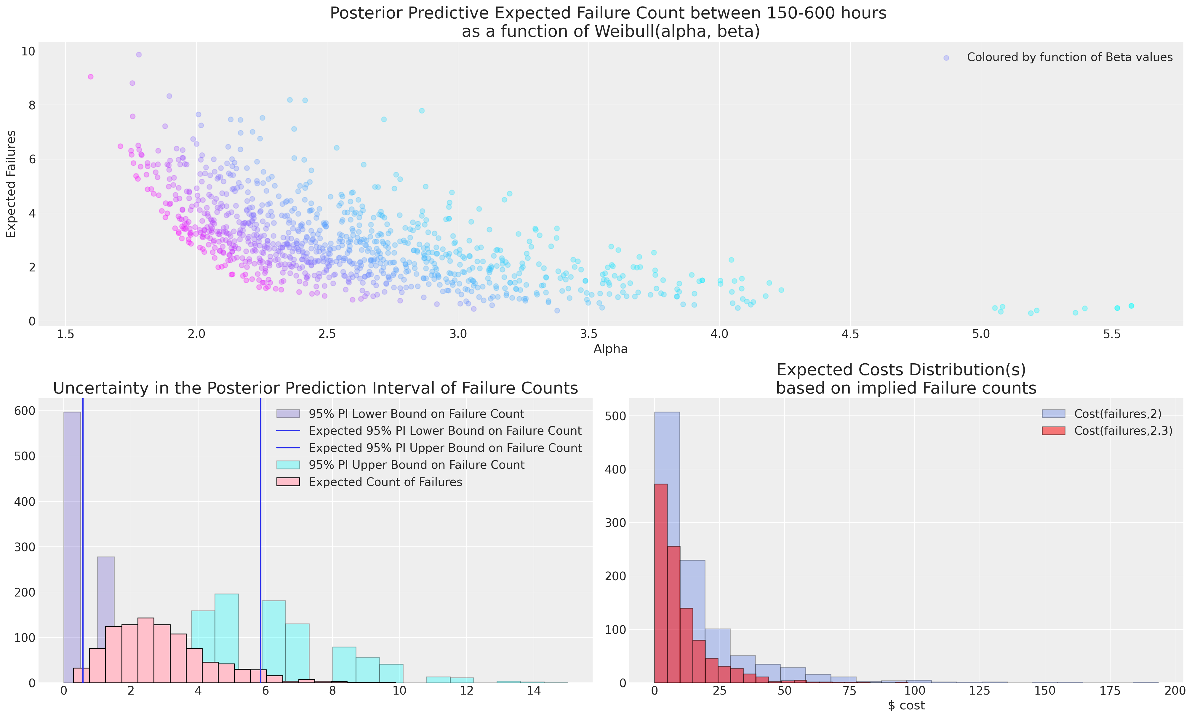
在这种情况下,模型的选择至关重要。关于哪种失效模式合适的决定必须由专业领域的专家来指导,因为从如此稀疏的数据中进行推断总是有风险的。如果失效会带来实际成本,那么对不确定性的理解就至关重要,而专业领域的专家通常更有能力判断在600小时的服务中是否可以合理预期2次或7次失效。
结论#
我们已经从频率论和贝叶斯的角度探讨了如何分析和建模可靠性,并与非参数估计进行了比较。我们展示了如何通过自助法和贝叶斯方法为多个关键统计量推导预测区间。我们已经看到了通过重采样方法和信息先验规范来校准这些预测区间的方法。这些观点是互补的,选择适当的技术应由感兴趣问题的因素驱动,而不是某种意识形态的承诺。
特别是,我们已经看到如何将MLE拟合到我们的轴承数据中,提供了一种在贝叶斯分析中建立先验的合理初步猜测方法。我们还看到如何通过从隐含模型中推导出关键量,并对这些推论进行审查,来引出专业知识。贝叶斯预测区间的选择是根据我们对先验期望的校准,在我们没有先验期望的情况下,我们可以提供模糊或非信息性的先验。这些先验的推论可以再次根据适当的成本函数进行检查和分析。
参考资料#
W.Q. Meeker, L.A. Escobar, 和 F.G Pascual. 可靠性数据的统计方法. Wiley, 2022.
水印#
%load_ext watermark
%watermark -n -u -v -iv -w -p pytensor,xarray_einstats
Last updated: Sun Jan 15 2023

Python implementation: CPython
Python version       : 3.10.8
IPython version      : 8.7.0

pytensor       : 2.8.10
xarray_einstats: 0.5.0.dev0

pandas    : 1.5.2
pymc      : 5.0.0
matplotlib: 3.6.2
xarray    : 2022.12.0
numpy     : 1.24.0
arviz     : 0.13.0

Watermark: 2.3.1