诊断带有分歧的偏差推理#
from collections import defaultdict

import arviz as az
import matplotlib.pyplot as plt
import numpy as np
import pandas as pd
import pymc3 as pm

print(f"Running on PyMC3 v{pm.__version__}")
Running on PyMC3 v3.11.5
%config InlineBackend.figure_format = 'retina'
az.style.use("arviz-darkgrid")
SEED = [20100420, 20134234]
本笔记本是 Michael Betancourt 在 mc-stan 上的帖子 的 PyMC3 移植版。有关底层机制的详细解释,请查看原始帖子 诊断偏差推理与分歧 以及 Betancourt 的优秀论文 哈密顿蒙特卡洛的概念介绍。
贝叶斯统计学是关于构建模型并估计该模型中的参数。然而,对我们的概率模型进行简单或直接的参数化有时可能效果不佳,你可以查看Thomas Wiecki的博客文章,为什么层次模型既棒又棘手,以及贝叶斯方法,该文章在PyMC3中讨论了同样的问题。次优的参数化通常会导致采样速度变慢,更严重的是,会导致MCMC估计器的偏差。
更正式地,正如在原文中所解释的,诊断偏差推理与分歧:
马尔可夫链蒙特卡罗(MCMC)近似于关于给定目标分布的期望,
使用马尔可夫链的状态,\({q{0}, \ldots, q_{N} }\),
然而,这些估计量只有在链增长到无限长时,才能保证渐近准确性,
为了在应用分析中发挥作用,我们需要MCMC估计器能够足够快地收敛到真实的期望值,以便在我们耗尽有限的计算资源之前,它们能够达到合理的准确性。这种快速收敛需要强遍历性条件成立,特别是马尔可夫转移与目标分布之间的几何遍历性。几何遍历性通常是MCMC估计器遵循中心极限定理的必要条件,这不仅确保了即使在有限次迭代后它们也是无偏的,而且还允许我们使用MCMC标准误差来经验性地量化它们的精度。
不幸的是,对于任何非平凡的问题,证明几何遍历性是不可行的。相反,我们必须依赖于经验诊断方法,这些方法能够识别阻碍几何遍历性的障碍,从而确保MCMC估计器的良好行为。对于一般的马尔可夫转移和目标分布,已知最好的诊断方法是基于参数空间中从扩散点初始化的一组马尔可夫链的分割\(\hat{R}\)统计量;要做得更好,我们需要利用给定转移或目标分布的特定结构。
例如,哈密顿蒙特卡洛(Hamiltonian Monte Carlo)在这方面特别强大,因为其相对于任何目标分布的几何遍历性失败会表现为不同的行为,这些行为已被发展为敏感的诊断工具。其中一种行为是出现发散现象,这表明哈密顿马尔可夫链遇到了目标分布中曲率较高的区域,而这些区域它无法充分探索。
在本笔记本中,我们旨在识别PyMC3中的分歧及其潜在的病理。
八校模型#
八校数据集(Rubin 1981)的分层模型,如在 Stan 中所见:
其中 \(n \in \{1, \ldots, 8 \}\) 且 \(\{ y_{n}, \sigma_{n} \}\) 作为数据给出。
推断层次超参数,\(\mu\) 和 \(\sigma\),以及组级参数,\(\theta_{1}, \ldots, \theta_{8}\),使模型能够在组之间汇集数据并减少它们的后验方差。不幸的是,直接的中心化参数化也将后验分布压缩到一个特别具有挑战性的几何形状中,阻碍了几何遍历性,从而导致MCMC估计产生偏差。
一个居中的八所学校实现#
Stan 模型:
data {
  int<lower=0> J;
  real y[J];
  real<lower=0> sigma[J];
}

parameters {
  real mu;
  real<lower=0> tau;
  real theta[J];
}

model {
  mu ~ normal(0, 5);
  tau ~ cauchy(0, 5);
  theta ~ normal(mu, tau);
  y ~ normal(theta, sigma);
}
同样地,我们可以轻松地在 PyMC3 中实现它
with pm.Model() as Centered_eight:
    mu = pm.Normal("mu", mu=0, sigma=5)
    tau = pm.HalfCauchy("tau", beta=5)
    theta = pm.Normal("theta", mu=mu, sigma=tau, shape=J)
    obs = pm.Normal("obs", mu=theta, sigma=sigma, observed=y)
不幸的是,该模型的直接实现表现出一种病态的几何结构,阻碍了几何遍历性。更令人担忧的是,由此产生的偏差是微妙的,仅通过检查马尔可夫链可能并不明显。为了理解这种偏差,让我们首先考虑一个短的马尔可夫链,通常在计算效率是一个主要因素时使用,之后再考虑一个更长的马尔可夫链。
一个危险短的马尔可夫链#
with Centered_eight:
    short_trace = pm.sample(600, chains=2, random_seed=SEED)
/Users/reshamashaikh/miniforge3/envs/pymc-ex/lib/python3.10/site-packages/deprecat/classic.py:215: FutureWarning: In v4.0, pm.sample will return an `arviz.InferenceData` object instead of a `MultiTrace` by default. You can pass return_inferencedata=True or return_inferencedata=False to be safe and silence this warning.
  return wrapped_(*args_, **kwargs_)
Auto-assigning NUTS sampler...
Initializing NUTS using jitter+adapt_diag...
Multiprocess sampling (2 chains in 2 jobs)
NUTS: [theta, tau, mu]
Sampling 2 chains for 1_000 tune and 600 draw iterations (2_000 + 1_200 draws total) took 16 seconds.
There were 52 divergences after tuning. Increase `target_accept` or reparameterize.
The acceptance probability does not match the target. It is 0.4129320535021329, but should be close to 0.8. Try to increase the number of tuning steps.
There were 10 divergences after tuning. Increase `target_accept` or reparameterize.
The acceptance probability does not match the target. It is 0.6090970402923143, but should be close to 0.8. Try to increase the number of tuning steps.
The rhat statistic is larger than 1.4 for some parameters. The sampler did not converge.
The estimated number of effective samples is smaller than 200 for some parameters.
在原文中,应用了1200个样本的单链。然而,由于PyMC3中未实现分裂\(\hat{R}\),我们改为使用每个600个样本的2条链进行拟合。
Gelman-Rubin诊断\(\hat{R}\)没有显示出任何问题(值都接近1)。你可以尝试使用不同的种子重新运行模型,看看这种情况是否仍然成立。
az.summary(short_trace).round(2)
Got error No model on context stack. trying to find log_likelihood in translation.
/Users/reshamashaikh/miniforge3/envs/pymc-ex/lib/python3.10/site-packages/arviz/data/io_pymc3_3x.py:98: FutureWarning: Using `from_pymc3` without the model will be deprecated in a future release. Not using the model will return less accurate and less useful results. Make sure you use the model argument or call from_pymc3 within a model context.
  warnings.warn(
| mean | sd | hdi_3% | hdi_97% | mcse_mean | mcse_sd | ess_bulk | ess_tail | r_hat | |
|---|---|---|---|---|---|---|---|---|---|
| mu | 3.76 | 2.84 | -2.00 | 9.43 | 0.20 | 0.15 | 182.0 | 288.0 | 1.20 |
| theta[0] | 5.29 | 4.88 | -4.38 | 14.48 | 0.30 | 0.32 | 220.0 | 445.0 | 1.28 |
| theta[1] | 4.33 | 4.28 | -3.78 | 13.19 | 0.25 | 0.27 | 257.0 | 275.0 | 1.40 |
| theta[2] | 3.20 | 4.64 | -6.18 | 12.93 | 0.26 | 0.25 | 254.0 | 437.0 | 1.10 |
| theta[3] | 4.04 | 4.23 | -4.63 | 12.05 | 0.22 | 0.20 | 247.0 | 402.0 | 1.12 |
| theta[4] | 3.11 | 4.10 | -5.22 | 11.27 | 0.21 | 0.17 | 292.0 | 290.0 | 1.18 |
| theta[5] | 3.44 | 4.47 | -7.27 | 11.66 | 0.24 | 0.38 | 289.0 | 327.0 | 1.38 |
| theta[6] | 5.36 | 4.35 | -2.80 | 14.17 | 0.33 | 0.33 | 175.0 | 395.0 | 1.25 |
| theta[7] | 4.17 | 4.55 | -5.80 | 12.50 | 0.23 | 0.19 | 328.0 | 455.0 | 1.47 |
| tau | 3.26 | 2.78 | 0.62 | 8.13 | 1.01 | 0.74 | 4.0 | 6.0 | 1.58 |
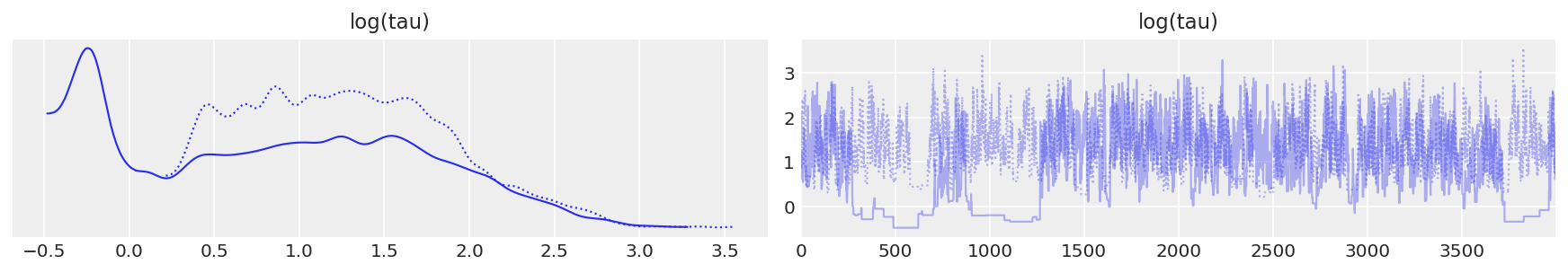
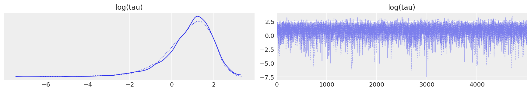
此外,所有轨迹图看起来都很好。让我们以分层标准差\(\tau\)为例,或者更具体地说,它的对数,\(log(\tau)\)。因为\(\tau\)被限制为正数,它的对数将使我们能够更好地解析小值的行为。实际上,链似乎在合理地探索小值和大值。
# plot the trace of log(tau)
ax = az.plot_trace(
    {"log(tau)": short_trace.get_values(varname="tau_log__", combine=False)}, legend=True
)
ax[0, 1].set_xlabel("Draw")
ax[0, 1].set_ylabel("log(tau)")
ax[0, 1].set_title("")

ax[0, 0].set_xlabel("log(tau)")
ax[0, 0].set_title("Probability density function of log(tau)");
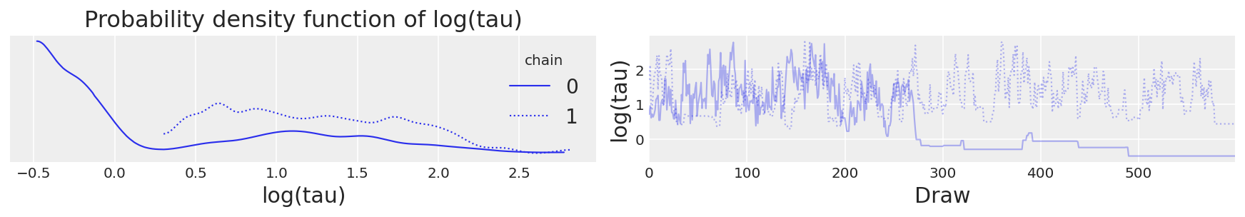
log(tau)的轨迹图#
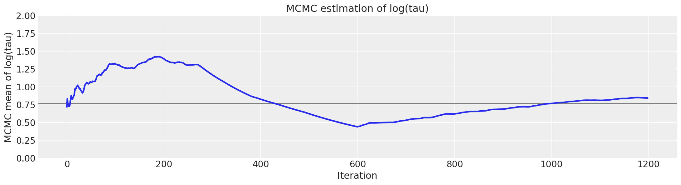
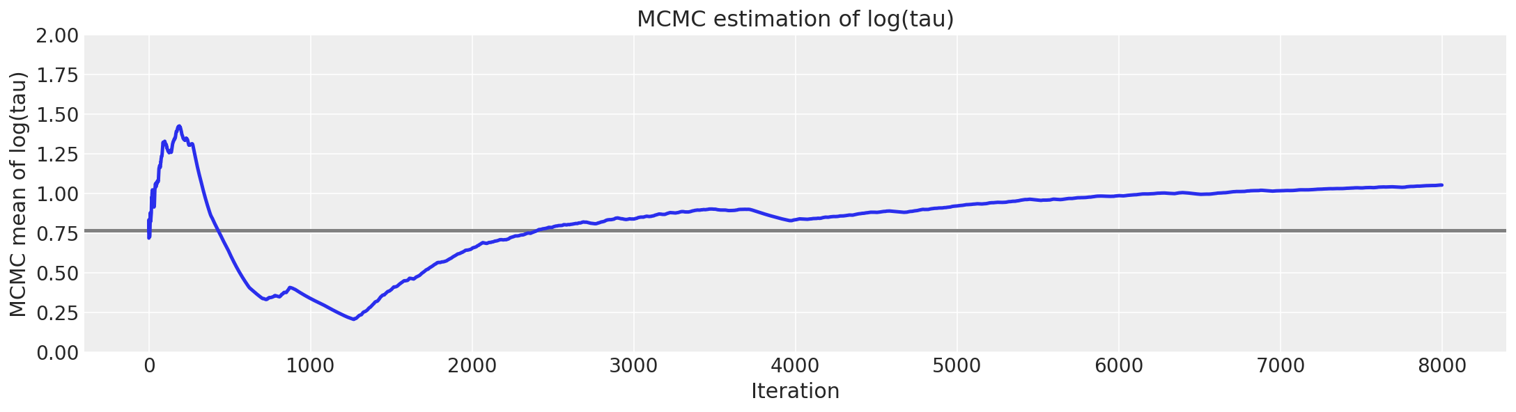
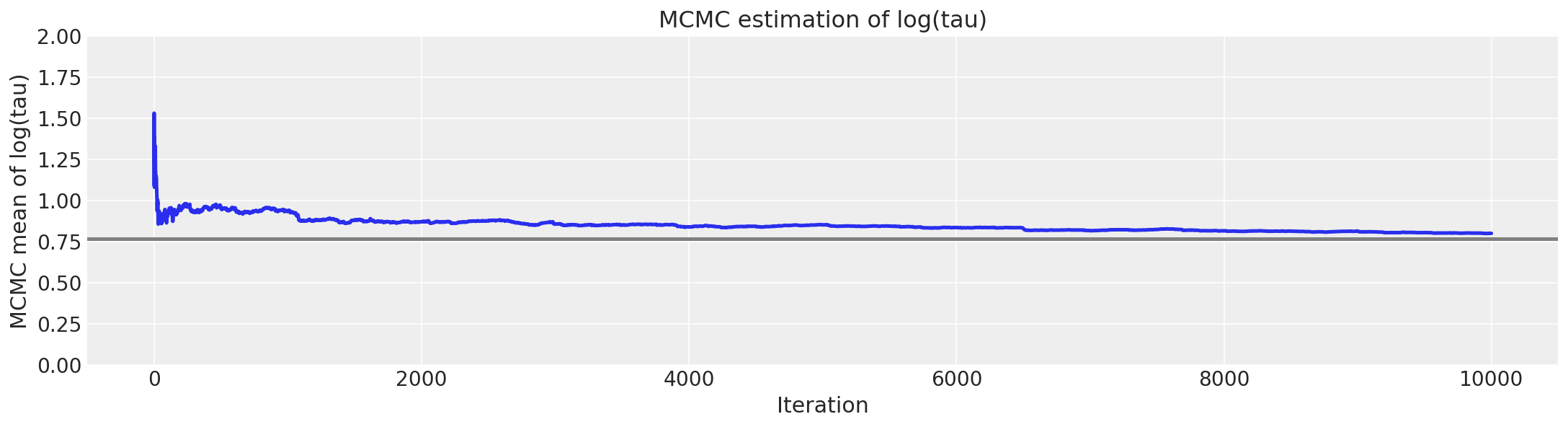
不幸的是,得到的\(log(\tau)\)均值估计值与真实值(此处以灰色显示)存在显著偏差。
# plot the estimate for the mean of log(τ) cumulating mean
logtau = np.log(short_trace["tau"])
mlogtau = [np.mean(logtau[:i]) for i in np.arange(1, len(logtau))]
plt.figure(figsize=(15, 4))
plt.axhline(0.7657852, lw=2.5, color="gray")
plt.plot(mlogtau, lw=2.5)
plt.ylim(0, 2)
plt.xlabel("Iteration")
plt.ylabel("MCMC mean of log(tau)")
plt.title("MCMC estimation of log(tau)");
然而,哈密顿蒙特卡洛(Hamiltonian Monte Carlo)并不像我们想象的那么忽视这些问题,因为在我们单独的马尔可夫链中,大约有3%的迭代以发散结束。
# display the total number and percentage of divergent
divergent = short_trace["diverging"]
print("Number of Divergent %d" % divergent.nonzero()[0].size)
divperc = divergent.nonzero()[0].size / len(short_trace) * 100
print("Percentage of Divergent %.1f" % divperc)
Number of Divergent 62
Percentage of Divergent 10.3
即使只有一条短链,这些分歧也能够识别偏差,并对任何由此产生的MCMC估计值持怀疑态度。
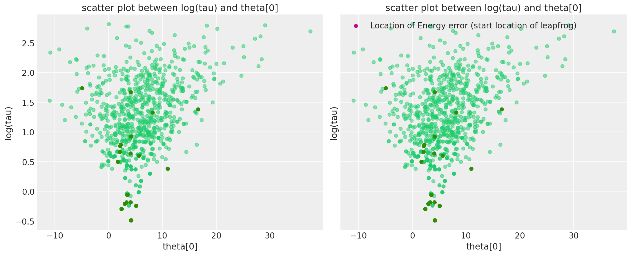
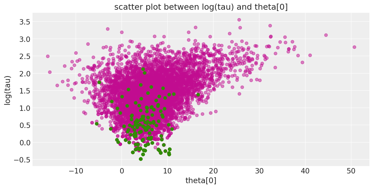
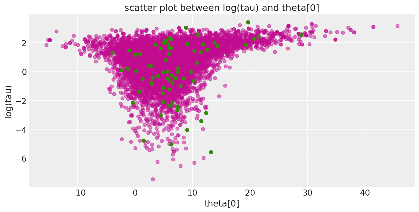
此外,由于发散的过渡(这里以绿色显示)往往位于病理附近,我们可以利用它们来识别参数空间中存在问题的邻域位置。
def pairplot_divergence(trace, ax=None, divergence=True, color="C3", divergence_color="C2"):
    theta = trace.get_values(varname="theta", combine=True)[:, 0]
    logtau = trace.get_values(varname="tau_log__", combine=True)
    if not ax:
        _, ax = plt.subplots(1, 1, figsize=(10, 5))
    ax.plot(theta, logtau, "o", color=color, alpha=0.5)
    if divergence:
        divergent = trace["diverging"]
        ax.plot(theta[divergent], logtau[divergent], "o", color=divergence_color)
    ax.set_xlabel("theta[0]")
    ax.set_ylabel("log(tau)")
    ax.set_title("scatter plot between log(tau) and theta[0]")
    return ax


pairplot_divergence(short_trace);
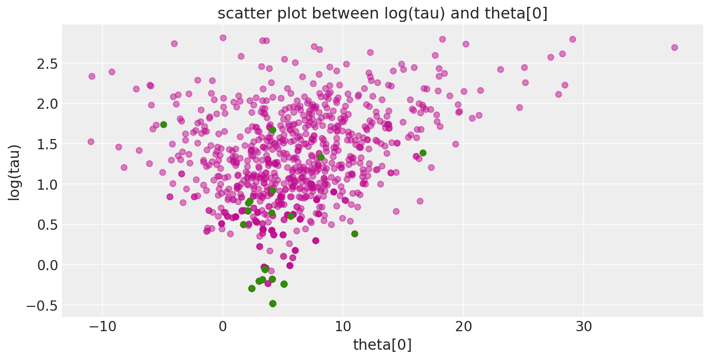
需要指出的是,来自轨迹的病理样本不一定集中在漏斗处:当遇到分歧时,正在构建的子树被拒绝,并且从现有的离散轨迹中均匀地采样过渡样本。因此,分歧样本不会精确地位于高曲率区域。
在 pymc3 中,我们最近实现了一个警告系统,该系统还会保存发散发生的位置信息,因此您可以直接可视化它们。更准确地说,我们在警告中包含的发散点是问题跳跃步开始的位置。有些可能是因为发散发生在其中一个跳跃步中(严格来说不是一个点)。但无论如何,可视化这些应该能更接近漏斗的位置。
注意,仅存储前100个分歧,以免占用所有内存。
divergent_point = defaultdict(list)

chain_warn = short_trace.report._chain_warnings
for i in range(len(chain_warn)):
    for warning_ in chain_warn[i]:
        if warning_.step is not None and warning_.extra is not None:
            for RV in Centered_eight.free_RVs:
                para_name = RV.name
                divergent_point[para_name].append(warning_.extra[para_name])

for RV in Centered_eight.free_RVs:
    para_name = RV.name
    divergent_point[para_name] = np.asarray(divergent_point[para_name])

tau_log_d = divergent_point["tau_log__"]
theta0_d = divergent_point["theta"]
Ndiv_recorded = len(tau_log_d)
_, ax = plt.subplots(1, 2, figsize=(15, 6), sharex=True, sharey=True)

pairplot_divergence(short_trace, ax=ax[0], color="C7", divergence_color="C2")

plt.title("scatter plot between log(tau) and theta[0]")

pairplot_divergence(short_trace, ax=ax[1], color="C7", divergence_color="C2")

theta_trace = short_trace["theta"]
theta0 = theta_trace[:, 0]

ax[1].plot(
    [theta0[divergent == 1][:Ndiv_recorded], theta0_d],
    [logtau[divergent == 1][:Ndiv_recorded], tau_log_d],
    "k-",
    alpha=0.5,
)

ax[1].scatter(
    theta0_d, tau_log_d, color="C3", label="Location of Energy error (start location of leapfrog)"
)

plt.title("scatter plot between log(tau) and theta[0]")
plt.legend();
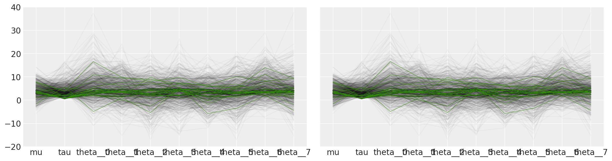
在参数空间中探索和可视化病理区域还有许多其他方法。例如,我们可以重现贝叶斯工作流中的可视化中的图5b。
tracedf = pm.trace_to_dataframe(short_trace)
plotorder = [
    "mu",
    "tau",
    "theta__0",
    "theta__1",
    "theta__2",
    "theta__3",
    "theta__4",
    "theta__5",
    "theta__6",
    "theta__7",
]
tracedf = tracedf[plotorder]

_, ax = plt.subplots(1, 2, figsize=(15, 4), sharex=True, sharey=True)
ax[0].plot(tracedf.values[divergent == 0].T, color="k", alpha=0.025)
ax[0].plot(tracedf.values[divergent == 1].T, color="C2", lw=0.5)

ax[1].plot(tracedf.values[divergent == 0].T, color="k", alpha=0.025)
ax[1].plot(tracedf.values[divergent == 1].T, color="C2", lw=0.5)
divsp = np.hstack(
    [
        divergent_point["mu"],
        np.exp(divergent_point["tau_log__"]),
        divergent_point["theta"],
    ]
)
ax[1].plot(divsp.T, "C3", lw=0.5)
plt.ylim([-20, 40])
plt.xticks(range(10), plotorder)
plt.tight_layout()
/var/folders/f5/4hllfzqx6pq2sfm22_khf5400000gn/T/ipykernel_63426/2369948333.py:32: UserWarning: This figure was using constrained_layout, but that is incompatible with subplots_adjust and/or tight_layout; disabling constrained_layout.
  plt.tight_layout()
# A small wrapper function for displaying the MCMC sampler diagnostics as above
def report_trace(trace):
    # plot the trace of log(tau)
    az.plot_trace({"log(tau)": trace.get_values(varname="tau_log__", combine=False)})

    # plot the estimate for the mean of log(τ) cumulating mean
    logtau = np.log(trace["tau"])
    mlogtau = [np.mean(logtau[:i]) for i in np.arange(1, len(logtau))]
    plt.figure(figsize=(15, 4))
    plt.axhline(0.7657852, lw=2.5, color="gray")
    plt.plot(mlogtau, lw=2.5)
    plt.ylim(0, 2)
    plt.xlabel("Iteration")
    plt.ylabel("MCMC mean of log(tau)")
    plt.title("MCMC estimation of log(tau)")
    plt.show()

    # display the total number and percentage of divergent
    divergent = trace["diverging"]
    print("Number of Divergent %d" % divergent.nonzero()[0].size)
    divperc = divergent.nonzero()[0].size / len(trace) * 100
    print("Percentage of Divergent %.1f" % divperc)

    # scatter plot between log(tau) and theta[0]
    # for the identification of the problematic neighborhoods in parameter space
    pairplot_divergence(trace);
一个更安全、更长的马尔可夫链#
鉴于分割\(\hat{R}\)对单个短链的潜在不敏感性,Stan建议尽可能运行多个链,以最大限度地观察到几何遍历性的任何障碍。然而,由于复杂模型并不总是能够运行长链,因此发散性是用于偏差MCMC估计的非常强大的诊断工具。
with Centered_eight:
    longer_trace = pm.sample(4000, chains=2, tune=1000, random_seed=SEED)
/Users/reshamashaikh/miniforge3/envs/pymc-ex/lib/python3.10/site-packages/deprecat/classic.py:215: FutureWarning: In v4.0, pm.sample will return an `arviz.InferenceData` object instead of a `MultiTrace` by default. You can pass return_inferencedata=True or return_inferencedata=False to be safe and silence this warning.
  return wrapped_(*args_, **kwargs_)
Auto-assigning NUTS sampler...
Initializing NUTS using jitter+adapt_diag...
Multiprocess sampling (2 chains in 2 jobs)
NUTS: [theta, tau, mu]
Sampling 2 chains for 1_000 tune and 4_000 draw iterations (2_000 + 8_000 draws total) took 56 seconds.
There were 224 divergences after tuning. Increase `target_accept` or reparameterize.
The acceptance probability does not match the target. It is 0.5963528759316614, but should be close to 0.8. Try to increase the number of tuning steps.
There were 66 divergences after tuning. Increase `target_accept` or reparameterize.
The acceptance probability does not match the target. It is 0.614889465736071, but should be close to 0.8. Try to increase the number of tuning steps.
The rhat statistic is larger than 1.05 for some parameters. This indicates slight problems during sampling.
The estimated number of effective samples is smaller than 200 for some parameters.
report_trace(longer_trace)
Number of Divergent 290
Percentage of Divergent 7.2
az.summary(longer_trace).round(2)
Got error No model on context stack. trying to find log_likelihood in translation.
/Users/reshamashaikh/miniforge3/envs/pymc-ex/lib/python3.10/site-packages/arviz/data/io_pymc3_3x.py:98: FutureWarning: Using `from_pymc3` without the model will be deprecated in a future release. Not using the model will return less accurate and less useful results. Make sure you use the model argument or call from_pymc3 within a model context.
  warnings.warn(
| mean | sd | hdi_3% | hdi_97% | mcse_mean | mcse_sd | ess_bulk | ess_tail | r_hat | |
|---|---|---|---|---|---|---|---|---|---|
| mu | 4.45 | 3.20 | -1.30 | 10.52 | 0.25 | 0.22 | 172.0 | 1723.0 | 1.01 |
| theta[0] | 6.42 | 5.63 | -2.97 | 18.08 | 0.20 | 0.14 | 497.0 | 2540.0 | 1.00 |
| theta[1] | 4.99 | 4.66 | -4.54 | 13.45 | 0.24 | 0.17 | 339.0 | 2300.0 | 1.01 |
| theta[2] | 3.97 | 5.33 | -6.64 | 13.66 | 0.25 | 0.18 | 302.0 | 2460.0 | 1.01 |
| theta[3] | 4.71 | 4.73 | -4.72 | 13.63 | 0.21 | 0.15 | 385.0 | 2574.0 | 1.01 |
| theta[4] | 3.65 | 4.60 | -5.26 | 12.23 | 0.26 | 0.18 | 272.0 | 2497.0 | 1.01 |
| theta[5] | 4.06 | 4.91 | -5.93 | 12.93 | 0.26 | 0.19 | 290.0 | 2266.0 | 1.00 |
| theta[6] | 6.36 | 4.96 | -1.99 | 16.76 | 0.15 | 0.10 | 771.0 | 2263.0 | 1.00 |
| theta[7] | 4.88 | 5.25 | -5.08 | 14.84 | 0.19 | 0.14 | 472.0 | 2634.0 | 1.01 |
| tau | 3.83 | 3.10 | 0.62 | 9.44 | 0.32 | 0.23 | 29.0 | 61.0 | 1.07 |
与Stan中的结果类似,\(\hat{R}\)并未表明任何严重问题。然而,每次迭代的有效样本量急剧下降,表明我们运行时间越长,探索效率越低。这种奇怪的行为清楚地表明某些问题正在发生。正如轨迹图所示,链在接近\(\tau\)的小值时偶尔会“卡住”,这正是我们看到发散集中的地方。这是一个明显的潜在病理迹象。这些粘滞区间在早期会导致MCMC估计器出现严重的振荡,直到它们最终稳定在有偏差的值上。
事实上,粘性区间是马尔可夫链试图纠正偏差探索的结果。如果我们运行链的时间更长,它最终会再次卡住,并将MCMC估计器拉向真实值。在无限次迭代的情况下,这种微妙的平衡会渐近地趋向于真实期望值,正如我们在MCMC的一致性保证下所预期的那样。然而,在任何有限次迭代后停止,都会破坏这种平衡,并留下显著的偏差。
更多详情可以在Betancourt的最新论文中找到。
通过调整PyMC3的适应程序来缓解分歧#
在哈密顿蒙特卡洛(Hamiltonian Monte Carlo)中,当哈密顿跃迁遇到曲率极大的区域时,例如层次漏斗的开口处,就会出现分歧。由于无法准确解析这些区域,跃迁功能失常并飞向无穷远。由于跃迁无法完全探索这些极端曲率的区域,我们失去了几何遍历性,并且我们的MCMC估计量变得有偏。
在Stan中实现的算法使用一种启发式方法来快速识别这些行为异常的轨迹,从而标记出分歧,而不必等待它们一直运行到无穷大。然而,这种启发式方法可能有点过于激进,有时会将转换标记为发散,即使我们并没有失去几何遍历性。
为了解决这种潜在的歧义,我们可以调整哈密顿跃迁的步长,\(\epsilon\)。步长越小,轨迹的准确性越高,越不容易被错误地标记为发散。换句话说,如果哈密顿跃迁和目标分布之间存在几何遍历性,那么减小步长将减少并最终完全消除发散。然而,如果我们没有几何遍历性,那么减小步长将不会完全消除发散。
与Stan类似,PyMC3中的步长在预热期间会自动调整,但我们可以通过调整PyMC3的自适应例程的配置来强制使用更小的步长。特别是,我们可以将target_accept参数从其默认值0.8增加到接近其最大值1。
调整适应程序#
with Centered_eight:
    fit_cp85 = pm.sample(5000, chains=2, tune=2000, target_accept=0.85)
/Users/reshamashaikh/miniforge3/envs/pymc-ex/lib/python3.10/site-packages/deprecat/classic.py:215: FutureWarning: In v4.0, pm.sample will return an `arviz.InferenceData` object instead of a `MultiTrace` by default. You can pass return_inferencedata=True or return_inferencedata=False to be safe and silence this warning.
  return wrapped_(*args_, **kwargs_)
Auto-assigning NUTS sampler...
Initializing NUTS using jitter+adapt_diag...
Multiprocess sampling (2 chains in 2 jobs)
NUTS: [theta, tau, mu]
Sampling 2 chains for 2_000 tune and 5_000 draw iterations (4_000 + 10_000 draws total) took 84 seconds.
There were 547 divergences after tuning. Increase `target_accept` or reparameterize.
The acceptance probability does not match the target. It is 0.4842846814954639, but should be close to 0.85. Try to increase the number of tuning steps.
There were 85 divergences after tuning. Increase `target_accept` or reparameterize.
The acceptance probability does not match the target. It is 0.737175456745239, but should be close to 0.85. Try to increase the number of tuning steps.
The rhat statistic is larger than 1.05 for some parameters. This indicates slight problems during sampling.
The estimated number of effective samples is smaller than 200 for some parameters.
with Centered_eight:
    fit_cp90 = pm.sample(5000, chains=2, tune=2000, target_accept=0.90)
/Users/reshamashaikh/miniforge3/envs/pymc-ex/lib/python3.10/site-packages/deprecat/classic.py:215: FutureWarning: In v4.0, pm.sample will return an `arviz.InferenceData` object instead of a `MultiTrace` by default. You can pass return_inferencedata=True or return_inferencedata=False to be safe and silence this warning.
  return wrapped_(*args_, **kwargs_)
Auto-assigning NUTS sampler...
Initializing NUTS using jitter+adapt_diag...
Multiprocess sampling (2 chains in 2 jobs)
NUTS: [theta, tau, mu]
Sampling 2 chains for 2_000 tune and 5_000 draw iterations (4_000 + 10_000 draws total) took 91 seconds.
There were 430 divergences after tuning. Increase `target_accept` or reparameterize.
The acceptance probability does not match the target. It is 0.705290719027636, but should be close to 0.9. Try to increase the number of tuning steps.
There were 74 divergences after tuning. Increase `target_accept` or reparameterize.
The rhat statistic is larger than 1.05 for some parameters. This indicates slight problems during sampling.
The estimated number of effective samples is smaller than 200 for some parameters.
with Centered_eight:
    fit_cp95 = pm.sample(5000, chains=2, tune=2000, target_accept=0.95)
/Users/reshamashaikh/miniforge3/envs/pymc-ex/lib/python3.10/site-packages/deprecat/classic.py:215: FutureWarning: In v4.0, pm.sample will return an `arviz.InferenceData` object instead of a `MultiTrace` by default. You can pass return_inferencedata=True or return_inferencedata=False to be safe and silence this warning.
  return wrapped_(*args_, **kwargs_)
Auto-assigning NUTS sampler...
Initializing NUTS using jitter+adapt_diag...
Multiprocess sampling (2 chains in 2 jobs)
NUTS: [theta, tau, mu]
Sampling 2 chains for 2_000 tune and 5_000 draw iterations (4_000 + 10_000 draws total) took 129 seconds.
There were 219 divergences after tuning. Increase `target_accept` or reparameterize.
The acceptance probability does not match the target. It is 0.8819302505195916, but should be close to 0.95. Try to increase the number of tuning steps.
There were 43 divergences after tuning. Increase `target_accept` or reparameterize.
The number of effective samples is smaller than 10% for some parameters.
with Centered_eight:
    fit_cp99 = pm.sample(5000, chains=2, tune=2000, target_accept=0.99)
/Users/reshamashaikh/miniforge3/envs/pymc-ex/lib/python3.10/site-packages/deprecat/classic.py:215: FutureWarning: In v4.0, pm.sample will return an `arviz.InferenceData` object instead of a `MultiTrace` by default. You can pass return_inferencedata=True or return_inferencedata=False to be safe and silence this warning.
  return wrapped_(*args_, **kwargs_)
Auto-assigning NUTS sampler...
Initializing NUTS using jitter+adapt_diag...
Multiprocess sampling (2 chains in 2 jobs)
NUTS: [theta, tau, mu]
Sampling 2 chains for 2_000 tune and 5_000 draw iterations (4_000 + 10_000 draws total) took 227 seconds.
There were 40 divergences after tuning. Increase `target_accept` or reparameterize.
The acceptance probability does not match the target. It is 0.9693984517210503, but should be close to 0.99. Try to increase the number of tuning steps.
There were 7 divergences after tuning. Increase `target_accept` or reparameterize.
The number of effective samples is smaller than 10% for some parameters.
df = pd.DataFrame(
    [
        longer_trace["step_size"].mean(),
        fit_cp85["step_size"].mean(),
        fit_cp90["step_size"].mean(),
        fit_cp95["step_size"].mean(),
        fit_cp99["step_size"].mean(),
    ],
    columns=["Step_size"],
)
df["Divergent"] = pd.Series(
    [
        longer_trace["diverging"].sum(),
        fit_cp85["diverging"].sum(),
        fit_cp90["diverging"].sum(),
        fit_cp95["diverging"].sum(),
        fit_cp99["diverging"].sum(),
    ]
)
df["delta_target"] = pd.Series([".80", ".85", ".90", ".95", ".99"])
df
| Step_size | Divergent | delta_target | |
|---|---|---|---|
| 0 | 0.276504 | 290 | .80 |
| 1 | 0.244083 | 632 | .85 |
| 2 | 0.164192 | 504 | .90 |
| 3 | 0.137629 | 262 | .95 |
| 4 | 0.043080 | 47 | .99 |
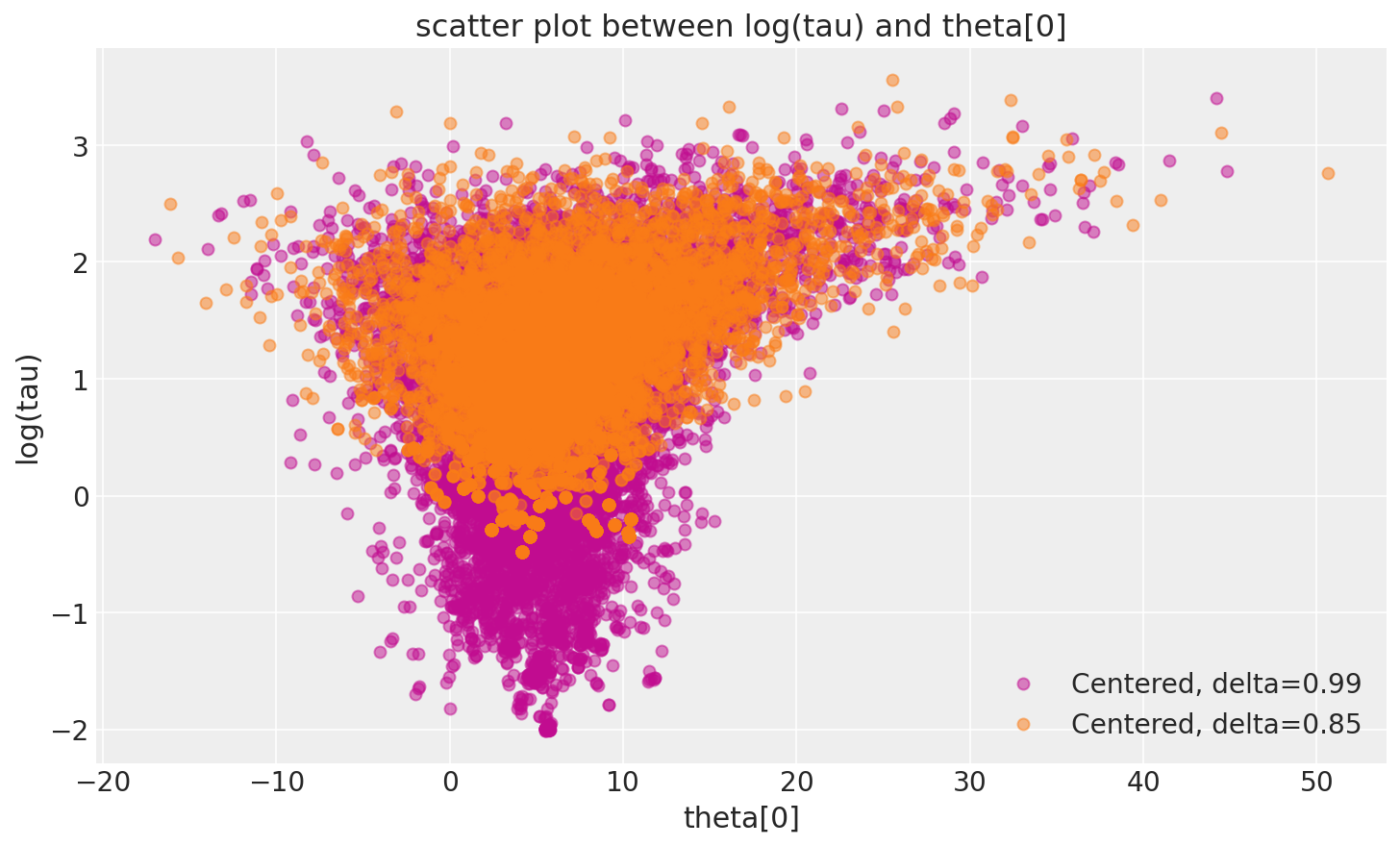
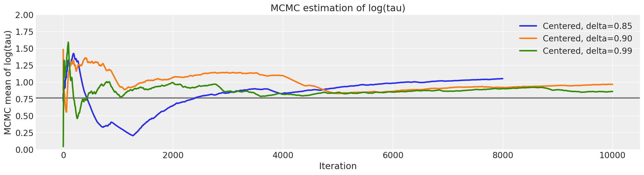
在这里,当delta增加到0.99时,发散过渡的数量急剧下降。
这种行为也有一个很好的几何直观。我们减少步长越多,哈密顿蒙特卡罗链就越能探索漏斗的颈部。因此,随着步长的减小,边缘后验分布\(log (\tau)\)会越来越向负值方向延伸。
由于在 PyMC3 中调参后步长比 Stan 更小,几何形状得到了更好的探索。
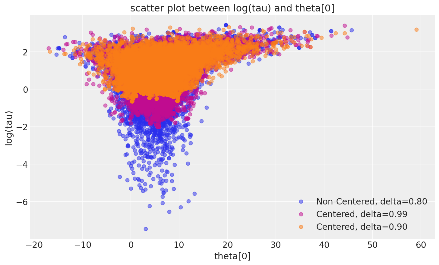
然而,哈密顿量转移在关于八校模型中心化实现方面仍然不是几何遍历的。实际上,鉴于观察到的偏差,这是可以预期的。
_, ax = plt.subplots(1, 1, figsize=(10, 6))

pairplot_divergence(fit_cp99, ax=ax, color="C3", divergence=False)

pairplot_divergence(longer_trace, ax=ax, color="C1", divergence=False)

ax.legend(["Centered, delta=0.99", "Centered, delta=0.85"]);
logtau0 = longer_trace["tau_log__"]
logtau2 = np.log(fit_cp90["tau"])
logtau1 = fit_cp99["tau_log__"]

plt.figure(figsize=(15, 4))
plt.axhline(0.7657852, lw=2.5, color="gray")
mlogtau0 = [np.mean(logtau0[:i]) for i in np.arange(1, len(logtau0))]
plt.plot(mlogtau0, label="Centered, delta=0.85", lw=2.5)
mlogtau2 = [np.mean(logtau2[:i]) for i in np.arange(1, len(logtau2))]
plt.plot(mlogtau2, label="Centered, delta=0.90", lw=2.5)
mlogtau1 = [np.mean(logtau1[:i]) for i in np.arange(1, len(logtau1))]
plt.plot(mlogtau1, label="Centered, delta=0.99", lw=2.5)
plt.ylim(0, 2)
plt.xlabel("Iteration")
plt.ylabel("MCMC mean of log(tau)")
plt.title("MCMC estimation of log(tau)")
plt.legend();
非中心化的八校实现#
尽管减小步长可以改善探索,但最终它只能揭示中心化实现中病理的真实程度。幸运的是,还有另一种实现分层模型的方法,不会受到相同的病理问题的影响。
在非中心化的参数化方法中,我们并不直接拟合组级别的参数,而是拟合一个潜在的高斯变量,通过缩放和平移我们可以从中恢复组级别的参数。
Stan 模型:
data {
  int<lower=0> J;
  real y[J];
  real<lower=0> sigma[J];
}

parameters {
  real mu;
  real<lower=0> tau;
  real theta_tilde[J];
}

transformed parameters {
  real theta[J];
  for (j in 1:J)
    theta[j] = mu + tau * theta_tilde[j];
}

model {
  mu ~ normal(0, 5);
  tau ~ cauchy(0, 5);
  theta_tilde ~ normal(0, 1);
  y ~ normal(theta, sigma);
}
with pm.Model() as NonCentered_eight:
    mu = pm.Normal("mu", mu=0, sigma=5)
    tau = pm.HalfCauchy("tau", beta=5)
    theta_tilde = pm.Normal("theta_t", mu=0, sigma=1, shape=J)
    theta = pm.Deterministic("theta", mu + tau * theta_tilde)
    obs = pm.Normal("obs", mu=theta, sigma=sigma, observed=y)
with NonCentered_eight:
    fit_ncp80 = pm.sample(5000, chains=2, tune=1000, random_seed=SEED, target_accept=0.80)
/Users/reshamashaikh/miniforge3/envs/pymc-ex/lib/python3.10/site-packages/deprecat/classic.py:215: FutureWarning: In v4.0, pm.sample will return an `arviz.InferenceData` object instead of a `MultiTrace` by default. You can pass return_inferencedata=True or return_inferencedata=False to be safe and silence this warning.
  return wrapped_(*args_, **kwargs_)
Auto-assigning NUTS sampler...
Initializing NUTS using jitter+adapt_diag...
Multiprocess sampling (2 chains in 2 jobs)
NUTS: [theta_t, tau, mu]
Sampling 2 chains for 1_000 tune and 5_000 draw iterations (2_000 + 10_000 draws total) took 32 seconds.
There were 19 divergences after tuning. Increase `target_accept` or reparameterize.
There were 52 divergences after tuning. Increase `target_accept` or reparameterize.
az.summary(fit_ncp80).round(2)
Got error No model on context stack. trying to find log_likelihood in translation.
/Users/reshamashaikh/miniforge3/envs/pymc-ex/lib/python3.10/site-packages/arviz/data/io_pymc3_3x.py:98: FutureWarning: Using `from_pymc3` without the model will be deprecated in a future release. Not using the model will return less accurate and less useful results. Make sure you use the model argument or call from_pymc3 within a model context.
  warnings.warn(
| mean | sd | hdi_3% | hdi_97% | mcse_mean | mcse_sd | ess_bulk | ess_tail | r_hat | |
|---|---|---|---|---|---|---|---|---|---|
| mu | 4.39 | 3.29 | -1.82 | 10.48 | 0.04 | 0.03 | 7993.0 | 4425.0 | 1.0 |
| theta_t[0] | 0.32 | 0.97 | -1.44 | 2.19 | 0.01 | 0.01 | 8723.0 | 5684.0 | 1.0 |
| theta_t[1] | 0.10 | 0.94 | -1.66 | 1.84 | 0.01 | 0.01 | 10767.0 | 6229.0 | 1.0 |
| theta_t[2] | -0.10 | 0.96 | -1.94 | 1.68 | 0.01 | 0.01 | 9773.0 | 5893.0 | 1.0 |
| theta_t[3] | 0.08 | 0.95 | -1.75 | 1.83 | 0.01 | 0.01 | 10138.0 | 6101.0 | 1.0 |
| theta_t[4] | -0.17 | 0.92 | -1.91 | 1.60 | 0.01 | 0.01 | 8721.0 | 6476.0 | 1.0 |
| theta_t[5] | -0.07 | 0.94 | -1.85 | 1.67 | 0.01 | 0.01 | 11379.0 | 7066.0 | 1.0 |
| theta_t[6] | 0.36 | 0.96 | -1.47 | 2.13 | 0.01 | 0.01 | 9317.0 | 6189.0 | 1.0 |
| theta_t[7] | 0.07 | 0.98 | -1.72 | 1.94 | 0.01 | 0.01 | 11444.0 | 6889.0 | 1.0 |
| tau | 3.64 | 3.36 | 0.00 | 9.39 | 0.05 | 0.04 | 4430.0 | 3569.0 | 1.0 |
| theta[0] | 6.26 | 5.57 | -4.45 | 16.36 | 0.07 | 0.06 | 6821.0 | 4801.0 | 1.0 |
| theta[1] | 4.93 | 4.55 | -3.61 | 13.80 | 0.05 | 0.04 | 9825.0 | 6967.0 | 1.0 |
| theta[2] | 3.84 | 5.30 | -5.75 | 14.24 | 0.07 | 0.06 | 7421.0 | 5379.0 | 1.0 |
| theta[3] | 4.86 | 4.85 | -3.93 | 14.24 | 0.05 | 0.05 | 8766.0 | 6023.0 | 1.0 |
| theta[4] | 3.57 | 4.64 | -5.70 | 11.97 | 0.05 | 0.04 | 8191.0 | 5926.0 | 1.0 |
| theta[5] | 4.02 | 4.90 | -4.93 | 13.28 | 0.06 | 0.05 | 7713.0 | 6105.0 | 1.0 |
| theta[6] | 6.35 | 4.99 | -2.62 | 16.06 | 0.06 | 0.04 | 8799.0 | 5610.0 | 1.0 |
| theta[7] | 4.92 | 5.33 | -4.54 | 15.72 | 0.06 | 0.04 | 8565.0 | 6393.0 | 1.0 |
如上所示,每次迭代的有效样本量有了显著的提升,轨迹图不再显示任何“粘滞性”。然而,我们仍然可以看到罕见的分歧。这些不频繁的分歧似乎并没有集中在参数空间的任何地方,这表明这些分歧可能是假阳性。
report_trace(fit_ncp80)
Number of Divergent 71
Percentage of Divergent 1.4
正如预期的那样,通过减小步长,我们可以完全消除这些假阳性。
with NonCentered_eight:
    fit_ncp90 = pm.sample(5000, chains=2, tune=1000, random_seed=SEED, target_accept=0.90)

# display the total number and percentage of divergent
divergent = fit_ncp90["diverging"]
print("Number of Divergent %d" % divergent.nonzero()[0].size)
/Users/reshamashaikh/miniforge3/envs/pymc-ex/lib/python3.10/site-packages/deprecat/classic.py:215: FutureWarning: In v4.0, pm.sample will return an `arviz.InferenceData` object instead of a `MultiTrace` by default. You can pass return_inferencedata=True or return_inferencedata=False to be safe and silence this warning.
  return wrapped_(*args_, **kwargs_)
Auto-assigning NUTS sampler...
Initializing NUTS using jitter+adapt_diag...
Multiprocess sampling (2 chains in 2 jobs)
NUTS: [theta_t, tau, mu]
Sampling 2 chains for 1_000 tune and 5_000 draw iterations (2_000 + 10_000 draws total) took 35 seconds.
There was 1 divergence after tuning. Increase `target_accept` or reparameterize.
Number of Divergent 1
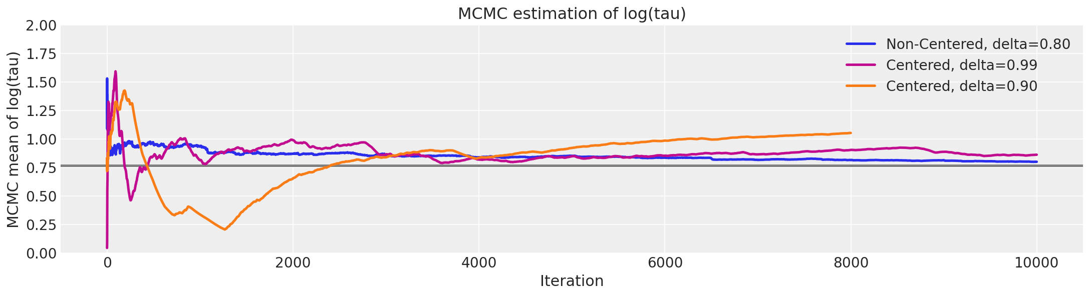
非中心化实现的更令人愉悦的几何结构使得马尔可夫链能够深入探索漏斗的颈部,捕捉到与测量结果一致的最小tau(\(\tau\))值。因此,非中心化链的MCMC估计器迅速收敛到其真实期望值。
_, ax = plt.subplots(1, 1, figsize=(10, 6))

pairplot_divergence(fit_ncp80, ax=ax, color="C0", divergence=False)
pairplot_divergence(fit_cp99, ax=ax, color="C3", divergence=False)
pairplot_divergence(fit_cp90, ax=ax, color="C1", divergence=False)

ax.legend(["Non-Centered, delta=0.80", "Centered, delta=0.99", "Centered, delta=0.90"]);
logtaun = fit_ncp80["tau_log__"]

plt.figure(figsize=(15, 4))
plt.axhline(0.7657852, lw=2.5, color="gray")
mlogtaun = [np.mean(logtaun[:i]) for i in np.arange(1, len(logtaun))]
plt.plot(mlogtaun, color="C0", lw=2.5, label="Non-Centered, delta=0.80")

mlogtau1 = [np.mean(logtau1[:i]) for i in np.arange(1, len(logtau1))]
plt.plot(mlogtau1, color="C3", lw=2.5, label="Centered, delta=0.99")

mlogtau0 = [np.mean(logtau0[:i]) for i in np.arange(1, len(logtau0))]
plt.plot(mlogtau0, color="C1", lw=2.5, label="Centered, delta=0.90")
plt.ylim(0, 2)
plt.xlabel("Iteration")
plt.ylabel("MCMC mean of log(tau)")
plt.title("MCMC estimation of log(tau)")
plt.legend();