


使用数据容器#
import warnings

import arviz as az
import matplotlib.pyplot as plt
import numpy as np
import pandas as pd
import pymc as pm

from numpy.random import default_rng

plt.rcParams["figure.constrained_layout.use"] = True

print(f"Running on PyMC v{pm.__version__}")
Running on PyMC v5.16.2
%matplotlib inline
%config InlineBackend.figure_format = 'retina'
RANDOM_SEED = sum(map(ord, "Data Containers in PyMC"))
rng = default_rng(RANDOM_SEED)
az.style.use("arviz-darkgrid")
介绍#
在构建了你梦想中的统计模型之后,你需要给它提供一些数据。数据通常以两种方式之一引入PyMC模型。一些数据作为外生输入使用,在线性回归模型中称为X,其中mu = X @ beta。其他数据是模型内生输出的“观察”示例,在回归模型中称为y,并作为输入用于模型隐含的似然函数。这些数据,无论是外生的还是内生的,都可以以多种数据类型包含在你的模型中,包括numpy ndarrays、pandas Series和DataFrame,甚至是pytensor TensorVariables。
尽管你可以将这些“原始”数据类型传递给你的 PyMC 模型,但将数据引入模型的最佳方式是使用 pymc.Data 容器。这些容器使得在 PyMC 模型中处理数据变得非常容易。它们提供了多种好处,包括:
将数据可视化作为概率图的一个组成部分
访问带标签的维度以提高可读性和可访问性
支持用于样本外预测、插值/外推、预测等的数据交换。
所有数据将存储在您的
arviz.InferenceData中,这对于绘图和可重复的工作流程非常有用。
本笔记本将依次说明这些好处,并向您展示将数据整合到您的PyMC建模工作流程中的最佳方法。
重要
在过去的PyMC版本中,有两种类型的数据容器 pymc.MutableData() 和 pymc.ConstantData()。这些已经被弃用,因为现在所有的数据容器都是可变的。
使用数据容器以提高可读性和可重复性#
该示例展示了使用数据容器与“原始”数据之间的一些差异。第一个模型展示了如何将原始数据(在此例中为numpy数组)直接提供给PyMC模型。
true_beta = 3
true_std = 5
n_obs = 100
x = rng.normal(size=n_obs)
y = rng.normal(loc=true_beta * x, scale=true_std, size=n_obs)

with pm.Model() as no_data_model:
    beta = pm.Normal("beta")
    mu = pm.Deterministic("mu", beta * x)
    sigma = pm.Exponential("sigma", 1)
    obs = pm.Normal("obs", mu=mu, sigma=sigma, observed=y)
    idata = pm.sample(random_seed=RANDOM_SEED)
Auto-assigning NUTS sampler...
Initializing NUTS using jitter+adapt_diag...
Multiprocess sampling (4 chains in 4 jobs)
NUTS: [beta, sigma]
Sampling 4 chains for 1_000 tune and 1_000 draw iterations (4_000 + 4_000 draws total) took 1 seconds.
查看生成的计算图,obs 节点被涂成灰色,以表明它已经观察到了数据,在这种情况下是 y。但数据本身并未显示在图中,因此没有关于已观察到什么数据的提示。此外,x 数据在图中任何地方都没有出现,因此不明显的是,该模型使用了外生数据作为输入。
pm.model_to_graphviz(no_data_model)

此外,在 idata 中,PyMC 已经自动保存了观测到的(内生)y 数据,但没有保存外生的 x 数据。如果我们想保存这些推理数据以供重用,或者将其作为可重复研究包的一部分提供,我们必须确保单独包含 x 数据。
idata.observed_data
<xarray.Dataset> Size: 2kB
Dimensions:    (obs_dim_0: 100)
Coordinates:
  * obs_dim_0  (obs_dim_0) int64 800B 0 1 2 3 4 5 6 7 ... 93 94 95 96 97 98 99
Data variables:
    obs        (obs_dim_0) float64 800B -0.3966 -3.337 -7.844 ... -6.549 -0.8598
Attributes:
    created_at:                 2024-07-28T11:34:21.141826+00:00
    arviz_version:              0.19.0
    inference_library:          pymc
inference_library_version: 5.16.2在下一个模型中,我们创建一个 pymc.Data 容器来保存观测值,并将此容器传递给 observed。我们还创建一个 pymc.Data 容器来保存 x 数据:
Auto-assigning NUTS sampler...
Initializing NUTS using jitter+adapt_diag...
Multiprocess sampling (4 chains in 4 jobs)
NUTS: [beta, sigma]
Sampling 4 chains for 1_000 tune and 1_000 draw iterations (4_000 + 4_000 draws total) took 1 seconds.
因为我们使用了 pymc.Data 容器,数据现在出现在我们的概率图中。它位于 obs 的下游(因为 obs 变量“导致”了数据),以灰色阴影显示(因为它是观测值),并且具有特殊的圆角方形形状以强调它是数据。我们还看到 x_data 已添加到图中。
pm.model_to_graphviz(no_data_model)

最后,我们可以检查推理数据,以确认x数据也已存储在那里。现在,它是一个包含所有必要信息以重现我们模型的完整摘要。
idata.constant_data
<xarray.Dataset> Size: 3kB
Dimensions:       (x_data_dim_0: 100, y_data_dim_0: 100)
Coordinates:
  * x_data_dim_0  (x_data_dim_0) int64 800B 0 1 2 3 4 5 6 ... 94 95 96 97 98 99
  * y_data_dim_0  (y_data_dim_0) int64 800B 0 1 2 3 4 5 6 ... 94 95 96 97 98 99
Data variables:
    x_data        (x_data_dim_0) float64 800B -1.383 -0.2725 ... -1.745 -0.5087
    y_data        (y_data_dim_0) float64 800B -0.3966 -3.337 ... -6.549 -0.8598
Attributes:
    created_at:                 2024-07-28T11:34:24.969470+00:00
    arviz_version:              0.19.0
    inference_library:          pymc
inference_library_version: 5.16.2使用数据容器的命名维度#
命名维度是使用数据容器带来的另一个强大优势。数据容器允许用户跟踪多维数据的维度(如日期或城市)和坐标(如实际的日期时间或城市名称)。两者都允许您指定随机变量的维度和坐标名称,而不是以数字形式指定这些随机变量的形状。请注意,在前面的概率图中,所有节点x_data、mu、obs和y_data都被放在一个带有数字100的框中。读者自然会问:“100是什么?”。维度和坐标通过回答这个问题来帮助组织模型、变量和数据。
在下一个示例中,我们生成一个为期2个月的三座城市温度的合成数据集。然后,我们将使用命名维度和坐标来提高模型代码的可读性和可视化的质量。
df_data = pd.DataFrame(columns=["date"]).set_index("date")
dates = pd.date_range(start="2020-05-01", end="2020-07-01")

for city, mu in {"Berlin": 15, "San Marino": 18, "Paris": 16}.items():
    df_data[city] = rng.normal(loc=mu, size=len(dates))

df_data.index = dates
df_data.index.name = "date"
df_data.head()
| Berlin | San Marino | Paris | |
|---|---|---|---|
| date | |||
| 2020-05-01 | 15.401536 | 18.817801 | 16.836690 |
| 2020-05-02 | 13.575241 | 17.441153 | 14.407089 |
| 2020-05-03 | 14.808934 | 19.890369 | 15.616649 |
| 2020-05-04 | 16.071487 | 18.407539 | 15.396678 |
| 2020-05-05 | 15.505263 | 17.621143 | 16.723544 |
如上所述,pymc.Data 允许您为数据的维度赋予命名标签。这是通过在创建模型时,向 pymc.Model 的 coords 参数传递一个包含 dimension: coordinate 键值对的字典来实现的。
关于维度、坐标及其巨大优势的更多解释,我们鼓励您查看ArviZ文档。
这是一大段解释——让我们看看它是如何完成的!我们将使用一个分层模型:它假设欧洲大陆的平均温度,并将每个城市相对于大陆平均温度进行建模:
# The data has two dimensions: date and city
# The "coordinates" are the unique values that these dimensions can take
coords = {"date": df_data.index, "city": df_data.columns}
with pm.Model(coords=coords) as model:
    data = pm.Data("observed_temp", df_data, dims=("date", "city"))

    europe_mean = pm.Normal("europe_mean_temp", mu=15.0, sigma=3.0)
    city_offset = pm.Normal("city_offset", mu=0.0, sigma=3.0, dims="city")
    city_temperature = pm.Deterministic(
        "expected_city_temp", europe_mean + city_offset, dims="city"
    )

    sigma = pm.Exponential("sigma", 1)
    pm.Normal("temperature", mu=city_temperature, sigma=sigma, observed=data, dims=("date", "city"))

    idata = pm.sample(
        random_seed=RANDOM_SEED,
    )
Auto-assigning NUTS sampler...
Initializing NUTS using jitter+adapt_diag...
Multiprocess sampling (4 chains in 4 jobs)
NUTS: [europe_mean_temp, city_offset, sigma]
Sampling 4 chains for 1_000 tune and 1_000 draw iterations (4_000 + 4_000 draws total) took 6 seconds.
再次,我们可以查看由我们的模型隐含的概率图。与之前一样,相似的节点(或节点组)被分组在板块内。板块上标注了每个节点的维度。之前,我们有标签100,并问:“100是什么?”。现在我们看到,在我们的模型中,有3个城市和62个日期。每个城市都有自己的偏移量,它与一个组平均值一起,决定了估计的温度。最后,我们看到我们的数据实际上是一个二维矩阵。添加标注的维度极大地改善了我们概率模型的展示。
pm.model_to_graphviz(model)

我们看到模型确实记住了我们给它的坐标:
for k, v in model.coords.items():
    print(f"{k}: {v[:20]}")
date: (Timestamp('2020-05-01 00:00:00'), Timestamp('2020-05-02 00:00:00'), Timestamp('2020-05-03 00:00:00'), Timestamp('2020-05-04 00:00:00'), Timestamp('2020-05-05 00:00:00'), Timestamp('2020-05-06 00:00:00'), Timestamp('2020-05-07 00:00:00'), Timestamp('2020-05-08 00:00:00'), Timestamp('2020-05-09 00:00:00'), Timestamp('2020-05-10 00:00:00'), Timestamp('2020-05-11 00:00:00'), Timestamp('2020-05-12 00:00:00'), Timestamp('2020-05-13 00:00:00'), Timestamp('2020-05-14 00:00:00'), Timestamp('2020-05-15 00:00:00'), Timestamp('2020-05-16 00:00:00'), Timestamp('2020-05-17 00:00:00'), Timestamp('2020-05-18 00:00:00'), Timestamp('2020-05-19 00:00:00'), Timestamp('2020-05-20 00:00:00'))
city: ('Berlin', 'San Marino', 'Paris')
坐标会自动存储到 arviz.InferenceData 对象中:
idata.posterior.coords
Coordinates:
  * chain    (chain) int64 32B 0 1 2 3
  * draw     (draw) int64 8kB 0 1 2 3 4 5 6 7 ... 993 994 995 996 997 998 999
  * city     (city) <U10 120B 'Berlin' 'San Marino' 'Paris'
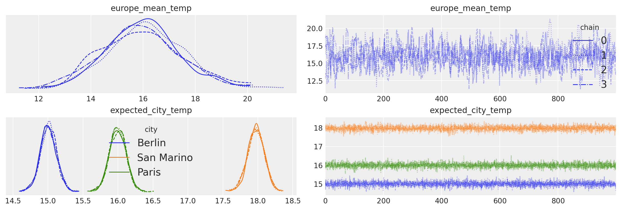
坐标在制作图表时也被arviz使用。在这里,我们将legend=True传递给az.plot_trace,以自动标记我们轨迹图中的三个城市。
axes = az.plot_trace(idata, var_names=["europe_mean_temp", "expected_city_temp"], legend=True);
当我们使用 pymc.Data 时,数据在内部表示为 pytensor 的 pytensor.tensor.sharedvar.TensorSharedVariable。
type(data)
pytensor.tensor.sharedvar.TensorSharedVariable
可以使用 pytensor.graph.Variable.eval() 方法检查所有 pytensor 张量的值。要访问数据,我们可以使用 pymc.Model 对象。所有模型变量,包括数据容器,都可以通过使用变量名称对模型对象本身进行索引来访问。由于这一行:
data = pm.Data("observed_temp", df_data, dims=("date", "city"))
将数据命名为“observed_temp”,我们可以按如下方式访问它:
model["observed_temp"].eval()[:15]
array([[15.40153619, 18.81780064, 16.83668986],
       [13.57524128, 17.4411525 , 14.40708945],
       [14.80893441, 19.89036942, 15.61664911],
       [16.07148689, 18.40753876, 15.39667778],
       [15.50526329, 17.62114292, 16.72354378],
       [14.86774578, 16.91297071, 16.64398094],
       [15.39861564, 18.06957647, 16.8952898 ],
       [14.82344668, 17.8925678 , 18.13033425],
       [14.29595165, 18.18139386, 14.87228836],
       [13.7296701 , 18.6225866 , 15.67262894],
       [14.68800267, 17.48605691, 15.26520975],
       [14.62891834, 19.16219466, 16.71921201],
       [14.58253668, 17.09701213, 17.10149473],
       [14.39255946, 17.66357467, 15.68899804],
       [15.8653625 , 16.66259542, 16.69857121]])
使用数据容器来改变数据#
在许多情况下,您会希望能够在模型运行之间切换数据。当您想要将模型拟合到多个数据集时,如果您对样本外预测感兴趣,以及在许多其他应用中,都会出现这种情况。
使用数据容器变量将同一模型拟合到多个数据集#
我们可以在PyMC中使用Data容器变量,将相同的模型拟合到多个数据集,而无需每次重新创建模型(如果数据集数量很大,这可能会非常耗时)。但请注意,每次模型仍将重新编译。
在下一个示例中,我们将生成10个具有单个参数mu的模型。每个模型将有一个不同观测数量的数据集,从10到100。我们将使用此设置来探索数据量对参数恢复的影响。
# We generate 10 datasets
n_models = 10
obs_multiplier = 10

true_mu = [rng.random() for _ in range(n_models)]
observed_data = [mu + rng.normal(size=(i + 1) * obs_multiplier) for i, mu in enumerate(true_mu)]

with pm.Model() as model:
    data = pm.Data("data", observed_data[0])
    mu = pm.Normal("mu", 0, 10)
    pm.Normal("y", mu=mu, sigma=1, observed=data)
正如我们之前所展示的,我们可以使用 eval 方法来检查我们的 Data 容器值:
model["data"].eval()
array([-0.10562792,  0.62102496,  1.48658991,  0.92295128,  0.43538261,
        0.73235925, -0.11983016,  0.89501808, -0.39242869,  1.4783441 ])
虽然可以使用eval来检查值,但使用pymc.set_data()来更改它们。让我们结合使用Data和pymc.set_data来将同一模型重复拟合到多个数据集上。请注意,每个数据集的大小不同并不重要!
# Generate one trace for each dataset
idatas = []
for data_vals in observed_data:
    with model:
        # Switch out the observed dataset
        pm.set_data({"data": data_vals})
        idatas.append(pm.sample(random_seed=RANDOM_SEED))
Show code cell output
Auto-assigning NUTS sampler...
Initializing NUTS using jitter+adapt_diag...
Multiprocess sampling (4 chains in 4 jobs)
NUTS: [mu]
Sampling 4 chains for 1_000 tune and 1_000 draw iterations (4_000 + 4_000 draws total) took 1 seconds.
Auto-assigning NUTS sampler...
Initializing NUTS using jitter+adapt_diag...
Multiprocess sampling (4 chains in 4 jobs)
NUTS: [mu]
Sampling 4 chains for 1_000 tune and 1_000 draw iterations (4_000 + 4_000 draws total) took 1 seconds.
Auto-assigning NUTS sampler...
Initializing NUTS using jitter+adapt_diag...
Multiprocess sampling (4 chains in 4 jobs)
NUTS: [mu]
Sampling 4 chains for 1_000 tune and 1_000 draw iterations (4_000 + 4_000 draws total) took 1 seconds.
Auto-assigning NUTS sampler...
Initializing NUTS using jitter+adapt_diag...
Multiprocess sampling (4 chains in 4 jobs)
NUTS: [mu]
Sampling 4 chains for 1_000 tune and 1_000 draw iterations (4_000 + 4_000 draws total) took 1 seconds.
Auto-assigning NUTS sampler...
Initializing NUTS using jitter+adapt_diag...
Multiprocess sampling (4 chains in 4 jobs)
NUTS: [mu]
Sampling 4 chains for 1_000 tune and 1_000 draw iterations (4_000 + 4_000 draws total) took 1 seconds.
Auto-assigning NUTS sampler...
Initializing NUTS using jitter+adapt_diag...
Multiprocess sampling (4 chains in 4 jobs)
NUTS: [mu]
Sampling 4 chains for 1_000 tune and 1_000 draw iterations (4_000 + 4_000 draws total) took 1 seconds.
Auto-assigning NUTS sampler...
Initializing NUTS using jitter+adapt_diag...
Multiprocess sampling (4 chains in 4 jobs)
NUTS: [mu]
Sampling 4 chains for 1_000 tune and 1_000 draw iterations (4_000 + 4_000 draws total) took 1 seconds.
Auto-assigning NUTS sampler...
Initializing NUTS using jitter+adapt_diag...
Multiprocess sampling (4 chains in 4 jobs)
NUTS: [mu]
Sampling 4 chains for 1_000 tune and 1_000 draw iterations (4_000 + 4_000 draws total) took 1 seconds.
Auto-assigning NUTS sampler...
Initializing NUTS using jitter+adapt_diag...
Multiprocess sampling (4 chains in 4 jobs)
NUTS: [mu]
Sampling 4 chains for 1_000 tune and 1_000 draw iterations (4_000 + 4_000 draws total) took 1 seconds.
Auto-assigning NUTS sampler...
Initializing NUTS using jitter+adapt_diag...
Multiprocess sampling (4 chains in 4 jobs)
NUTS: [mu]
Sampling 4 chains for 1_000 tune and 1_000 draw iterations (4_000 + 4_000 draws total) took 1 seconds.
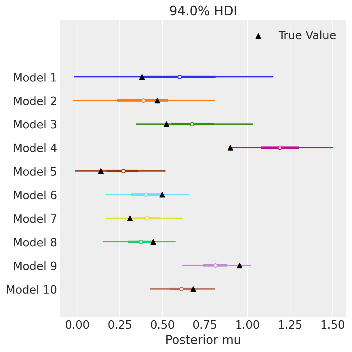
Arviz 的 arviz.plot_forest() 允许你传递一个包含相同变量名称的 idata 对象列表。通过这种方式,我们可以快速可视化来自10个不同数据集的不同估计值。我们还使用 matplotlib 在 plot_forest 上散布真实参数值。我们可以看到,随着我们从模型1中的10个观测值增加到模型10中的100个观测值,估计值越来越集中在mu的真实值上,并且估计值周围的误差逐渐减少。
model_idx = np.arange(n_models, dtype="int")
axes = az.plot_forest(idatas, var_names=["mu"], combined=True, figsize=(6, 6), legend=False)

ax = axes[0]
y_vals = np.stack([ax.get_lines()[i].get_ydata() for i in np.arange(n_models)]).ravel()
ax.scatter(true_mu, y_vals[::-1], marker="^", color="k", zorder=100, label="True Value")
ax.set(yticklabels=[f"Model {i+1}" for i in model_idx[::-1]], xlabel="Posterior mu")
ax.legend()
plt.show()
应用示例:使用数据容器作为二项式GLM的输入#
机器学习中的一个常见任务是为未见过的数据预测值,而 Data 容器变量正是我们完成这一任务所需的。
在这种情况下需要注意的一个小细节是,输入数据(x)和输出数据(obs)的形状必须相同。当我们进行样本外预测时,通常只改变输入数据,其形状可能与训练观测值不同。如果仅改变其中一个,将会导致形状错误。有两种解决方案:
使用
pymc.Data作为x数据和y数据,并使用pm.set_data将y更改为与测试输入相同形状的内容。告诉 PyMC,
obs的形状应始终与输入数据的形状相同。
在下一个模型中,我们使用选项2。这样,我们不需要每次更改x时都向y传递虚拟数据。
n_obs = 100
true_beta = 1.5
true_alpha = 0.25

x = rng.normal(size=n_obs)
true_p = 1 / (1 + np.exp(-(true_alpha + true_beta * x)))
y = rng.binomial(n=1, p=true_p)
with pm.Model() as logistic_model:
    x_data = pm.Data("x", x)
    y_data = pm.Data("y", y)

    alpha = pm.Normal("alpha")
    beta = pm.Normal("beta")

    p = pm.Deterministic("p", pm.math.sigmoid(alpha + beta * x_data))

    # Here is were we link the shapes of the inputs (x_data) and the observed varaiable
    # It will be the shape we tell it, rather than the (constant!) shape of y_data
    obs = pm.Bernoulli("obs", p=p, observed=y_data, shape=x_data.shape[0])

    # fit the model
    idata = pm.sample(random_seed=RANDOM_SEED)

    # Generate a counterfactual dataset using our model
    idata = pm.sample_posterior_predictive(
        idata, extend_inferencedata=True, random_seed=RANDOM_SEED
    )
Auto-assigning NUTS sampler...
Initializing NUTS using jitter+adapt_diag...
Multiprocess sampling (4 chains in 4 jobs)
NUTS: [alpha, beta]
Sampling 4 chains for 1_000 tune and 1_000 draw iterations (4_000 + 4_000 draws total) took 1 seconds.
Sampling: [obs]
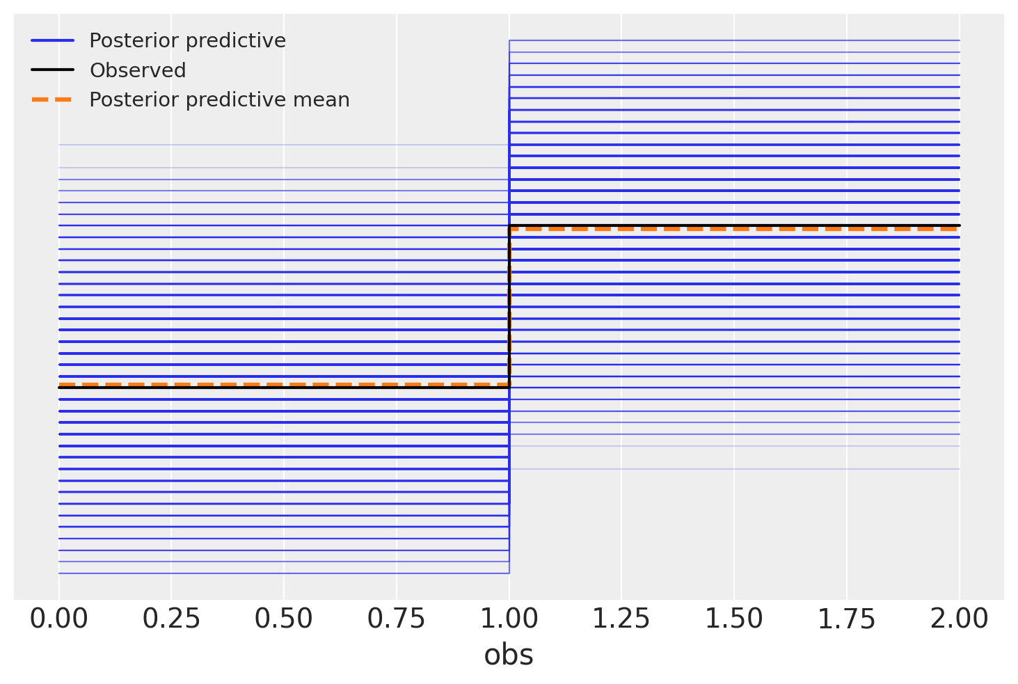
一个常见的后估计诊断方法是查看后验预测图,使用arviz.plot_ppc()。这显示了从模型中采样的数据的分布以及观测数据。如果它们看起来相似,我们就有一些证据表明模型并不差。
然而,在这种情况下,解释后验预测图可能会很困难。由于我们正在进行逻辑回归,观察到的值只能是零或一。因此,后验预测图呈现出俄罗斯方块块的形状。我们该如何理解这一点呢?显然,我们的模型产生的1比0多,平均比例与数据相符。但该比例也存在很大的不确定性。我们还能对模型的性能说些什么呢?
az.plot_ppc(idata)
<Axes: xlabel='obs'>
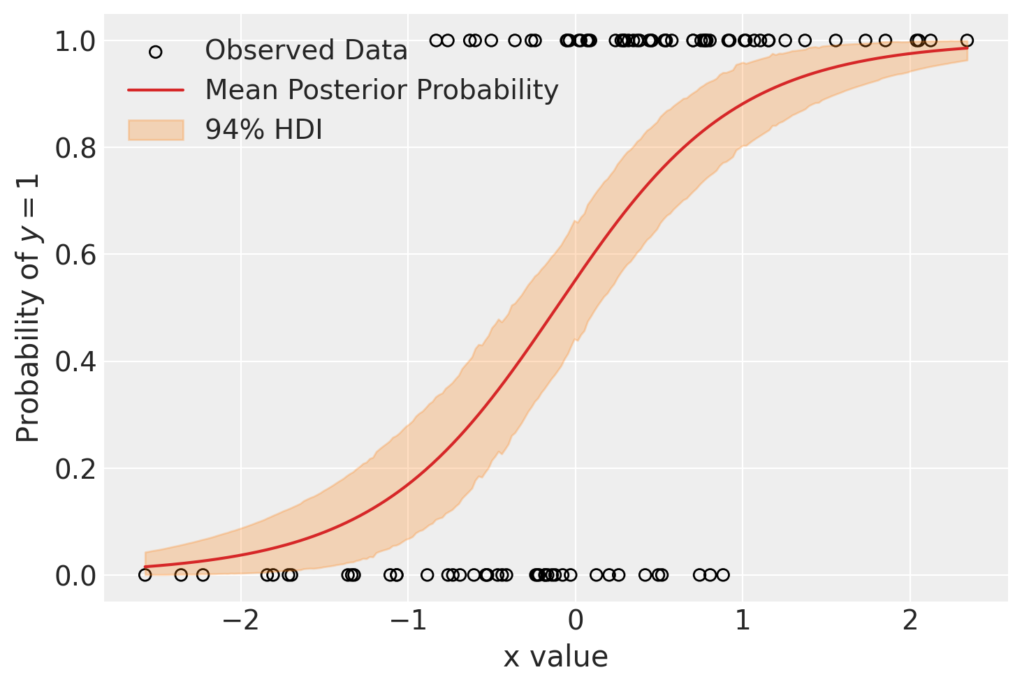
我们可以制作的另一个图表来查看模型的表现,是观察潜在变量 p 在协变量空间中的演变。我们期望协变量和数据之间存在某种关系,而我们的模型在变量 p 中编码了这种关系。在这个模型中,唯一的协变量是 x。如果 x 和 y 之间的关系是正向的,我们期望在 x 较小时,p 较低且观察到许多零,而在 x 较大时,p 较高且观察到许多一。
这很好,但用于绘图时,x 是混乱的。诚然,我们可以直接对值进行排序。但另一种方法(展示了如何使用我们的 Data!)是将均匀分布的 x 值网格传递到我们的模型中。这相当于在网格上的每个点对 p 进行预测,这将给我们一个很好的可绘制结果。这也是我们如何使用模型进行插值或外推的方法,所以这是一个非常值得了解的技巧。
在下一个代码块中,我们将x的(随机打乱的)值替换为均匀间隔的网格值,这些值跨越了观察到的x的范围。
grid_size = 250
x_grid = np.linspace(x.min(), x.max(), grid_size)
with logistic_model:
    # Switch out the observations and use `sample_posterior_predictive` to predict
    # We do not need to set data for the outputs because we told the model to always link the shape of the output to the shape
    # of the input.
    pm.set_data({"x": x_grid})
    post_idata = pm.sample_posterior_predictive(
        idata, var_names=["p", "obs"], random_seed=RANDOM_SEED
    )
Sampling: [obs]
使用新的 post_idata,其中包含 p 的样本外“预测”,我们绘制了 x_grid 与 p 的关系图。我们还绘制了观测数据。我们可以看到,模型在 x 较小时预期低概率 (p),并且概率随 x 的变化非常缓慢。
fig, ax = plt.subplots()
hdi = az.hdi(post_idata.posterior_predictive.p).p

ax.scatter(x, y, facecolor="none", edgecolor="k", label="Observed Data")
p_mean = post_idata.posterior_predictive.p.mean(dim=["chain", "draw"])
ax.plot(x_grid, p_mean, color="tab:red", label="Mean Posterior Probability")
ax.fill_between(x_grid, *hdi.values.T, color="tab:orange", alpha=0.25, label="94% HDI")
ax.legend()
ax.set(ylabel="Probability of $y=1$", xlabel="x value")
plt.show()
同样的概念应用于更复杂的模型可以在笔记本 变分推断:贝叶斯神经网络 中看到。
应用示例:幼儿身高作为年龄的函数#
此示例摘自Osvaldo Martin的书籍:《Python贝叶斯分析:使用PyMC和ArviZ进行统计建模和概率编程的介绍,第二版》 [Martin, 2018]。
世界卫生组织和世界各地的其他卫生机构收集新生儿和幼儿的数据,并设计生长曲线标准。这些图表是儿科工具包的重要组成部分,同时也是衡量人口整体健康状况的指标,以便制定健康政策、规划干预措施并监测其有效性。
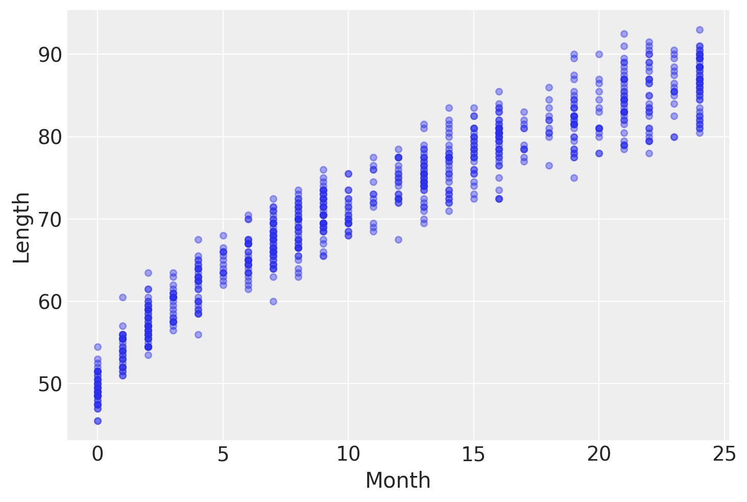
此类数据的一个例子是新生儿/幼儿女孩的身高随年龄(以月为单位)变化的数据:
try:
    data = pd.read_csv("../data/babies.csv")
except FileNotFoundError:
    data = pd.read_csv(pm.get_data("babies.csv"))
data.plot.scatter("Month", "Length", alpha=0.4);
为了对这些数据进行建模,我们需要对coords进行变异,因为数据索引需要根据测试数据集的索引进行更改。幸运的是,coords总是可变的,因此我们可以在样本外预测期间对其进行变异。
在示例中,我们将更新obs_idx的坐标,以反映测试数据集的索引。
with pm.Model(
    coords={"obs_idx": np.arange(len(data)), "parameter": ["intercept", "slope"]}
) as model_babies:
    mean_params = pm.Normal("mean_params", sigma=10, dims=["parameter"])
    sigma_params = pm.Normal("sigma_params", sigma=10, dims=["parameter"])
    month = pm.Data("month", data.Month.values.astype(float), dims=["obs_idx"])

    mu = pm.Deterministic("mu", mean_params[0] + mean_params[1] * month**0.5, dims=["obs_idx"])
    sigma = pm.Deterministic("sigma", sigma_params[0] + sigma_params[1] * month, dims=["obs_idx"])

    length = pm.Normal("length", mu=mu, sigma=sigma, observed=data.Length, dims=["obs_idx"])

    idata_babies = pm.sample(random_seed=RANDOM_SEED)
Auto-assigning NUTS sampler...
Initializing NUTS using jitter+adapt_diag...
Multiprocess sampling (4 chains in 4 jobs)
NUTS: [mean_params, sigma_params]
Sampling 4 chains for 1_000 tune and 1_000 draw iterations (4_000 + 4_000 draws total) took 2 seconds.
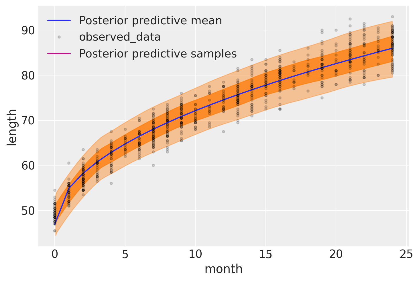
下图展示了我们模型的结果。期望长度,\(\mu\),用蓝色曲线表示,两个半透明的橙色带表示后验预测长度测量的60%和94%最高后验密度区间:
with model_babies:
    pm.sample_posterior_predictive(idata_babies, extend_inferencedata=True, random_seed=RANDOM_SEED)
Sampling: [length]
ax = az.plot_hdi(
    data.Month,
    idata_babies.posterior_predictive["length"],
    hdi_prob=0.6,
    fill_kwargs={"color": "tab:orange", "alpha": 0.8},
)
ax.plot(
    data.Month,
    idata_babies.posterior["mu"].mean(("chain", "draw")),
    label="Posterior predictive mean",
)
ax = az.plot_lm(
    idata=idata_babies,
    y="length",
    x="month",
    kind_pp="hdi",
    y_kwargs={"color": "k", "ms": 6, "alpha": 0.15},
    y_hat_fill_kwargs=dict(fill_kwargs={"color": "tab:orange", "alpha": 0.4}),
    axes=ax,
)
在撰写本文时,Osvaldo 的女儿刚满两周(\(\approx 0.5\) 个月),因此他想知道她的身高如何与我们刚刚创建的生长曲线进行比较。回答这个问题的一种方法是询问模型在 0.5 个月大的婴儿中变量长度的分布。使用 PyMC,我们可以通过函数 sample_posterior_predictive 来提出这个问题,因为它将返回基于观测数据和参数估计分布的 Length 样本,即包括不确定性。
唯一的问题是,默认情况下,此函数将返回月份的观测值对应的长度预测,而\(0.5\)个月(Osvaldo关心的值)并未被观测到——所有测量都是针对整数月份报告的。获取月份的非观测值预测的更简单方法是,将新值传递给我们之前在模型中定义的Data容器。为此,我们需要使用pm.set_data,然后只需从后验预测分布中采样即可。我们还需要为这些新观测值设置coords,我们可以在pm.set_data函数中这样做,因为我们已经将obs_idx坐标设置为可变的。
请注意,在这种情况下,我们为 obs_idx 传递的实际值是完全无关紧要的,因此我们给它赋值为 0。重要的是,我们将其更新为与我们要进行样本外预测的年龄长度相同,并且每个年龄都有一个唯一的索引标识符。
ages_to_check = [0.5]
with model_babies:
    pm.set_data({"month": ages_to_check}, coords={"obs_idx": [0]})

    # Setting predictions=True will add a new "predictions" group to our idata. This lets us store the posterior,
    # posterior_predictive, and predictions all in the same object.
    idata_babies = pm.sample_posterior_predictive(
        idata_babies, extend_inferencedata=True, predictions=True, random_seed=RANDOM_SEED
    )
Sampling: [length]
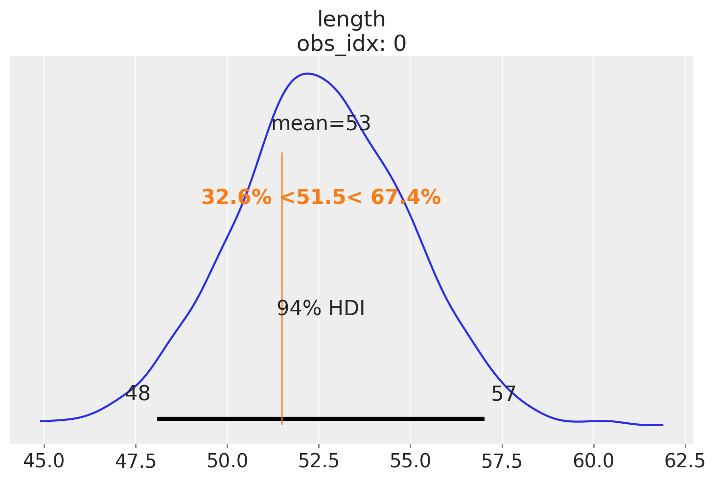
现在我们可以绘制2周大婴儿长度的预期分布图,并计算其他量——例如,给定她的长度,计算一个孩子的百分位数。这里,让我们假设我们感兴趣的孩子长度为51.5:
ref_length = 51.5

az.plot_posterior(
    idata_babies,
    group="predictions",
    ref_val={"length": [{"ref_val": ref_length}]},
    labeller=az.labels.DimCoordLabeller(),
);
参考资料#
Osvaldo Martin. 使用Python进行贝叶斯分析:使用PyMC3和ArviZ进行统计建模和概率编程的介绍. Packt Publishing Ltd, 2018.
水印#
%load_ext watermark
%watermark -n -u -v -iv -w -p pytensor,xarray
Last updated: Sun Jul 28 2024

Python implementation: CPython
Python version       : 3.12.4
IPython version      : 8.26.0

pytensor: 2.25.2
xarray  : 2024.6.0

arviz     : 0.19.0
numpy     : 1.26.4
pymc      : 5.16.2
matplotlib: 3.9.1
pandas    : 2.2.2

Watermark: 2.4.3