


二项回归#
本笔记本涵盖了二项回归背后的逻辑,这是广义线性模型的一个特定实例。示例保持非常简单,只有一个预测变量。
回顾逻辑回归有助于理解何时适用二项回归。逻辑回归在结果变量是一系列成功或失败,即一系列0、1观察值时非常有用。这种结果变量的一个例子是“你今天跑步了吗?”二项回归(又称聚合二项回归)在你有\(n\)次试验中的若干次成功时非常有用。因此,例子会是“在过去7天里,你有几天去跑步了?”
观察到的数据是一组在\(n\)次总试验中成功的计数。许多人可能会倾向于将这些数据简化为一个比例,但这并不一定是个好主意。例如,比例并不是直接测量的,它们通常最好被视为需要估计的潜在变量。此外,比例会丢失信息:0.5的比例可能对应于2天中的1次运行,或者过去4周中的4次运行,或者其他许多情况,但您通过只关注比例而丢失了这些信息。
二项回归的适当似然函数是二项分布:
其中 \(y_i\) 是 \(n\) 次试验中成功的次数,\(p_i\) 是成功的(潜在)概率。我们希望通过二项回归实现的是使用线性模型来准确估计 \(p_i\)(即 \(p_i = \beta_0 + \beta_1 \cdot x_i\))。因此,我们可以尝试使用类似以下的似然项来实现这一点:
如果我们这样做,当线性模型生成的值 \(p\) 超出 \(0-1\) 的范围时,我们很快就会遇到问题。这时就需要用到链接函数:
其中 \(g()\) 是一个链接函数。这可以被认为是一种将范围在 \((0, 1)\) 内的比例映射到 \((-\infty, +\infty)\) 域的变换。有许多可能的函数可以使用,但一个常用的函数是 Logit 函数。
尽管我们实际上想要做的是重新排列这个方程以得到\(p_i\),以便我们可以将其输入到似然函数中。这导致了:
其中 \(g^{-1}()\) 是链接函数的逆函数,在本例中是Logit函数的逆函数(即逻辑斯蒂Sigmoid函数,也称为expit函数)。因此,如果我们将此代入我们的似然函数,最终得到:
这定义了我们的似然函数。现在,您只需要对 \(\beta\) 参数设置先验,就可以进行贝叶斯二项回归了。观测数据是 \(y_i\)、\(n\) 和 \(x_i\)。
import arviz as az
import matplotlib.pyplot as plt
import numpy as np
import pandas as pd
import pymc as pm

from scipy.special import expit
%config InlineBackend.figure_format = 'retina'
az.style.use("arviz-darkgrid")
rng = np.random.default_rng(1234)
生成数据#
# true params
beta0_true = 0.7
beta1_true = 0.4
# number of yes/no questions
n = 20

sample_size = 30
x = np.linspace(-10, 20, sample_size)
# Linear model
mu_true = beta0_true + beta1_true * x
# transformation (inverse logit function = expit)
p_true = expit(mu_true)
# Generate data
y = rng.binomial(n, p_true)
# bundle data into dataframe
data = pd.DataFrame({"x": x, "y": y})
我们可以看到基础数据 \(y\) 是计数数据,来自总共 \(n\) 次试验。
data.head()
| x | y | |
|---|---|---|
| 0 | -10.000000 | 3 |
| 1 | -8.965517 | 1 |
| 2 | -7.931034 | 3 |
| 3 | -6.896552 | 1 |
| 4 | -5.862069 | 2 |
Show code cell source
# Plot underlying linear model
fig, ax = plt.subplots(2, 1, figsize=(9, 6), sharex=True)
ax[0].plot(x, mu_true, label=r"$β_0 + β_1 \cdot x_i$")
ax[0].set(xlabel="$x$", ylabel=r"$β_0 + β_1 \cdot x_i$", title="Underlying linear model")
ax[0].legend()

# Plot GLM
freq = ax[1].twinx()  # instantiate a second axes that shares the same x-axis
freq.set_ylabel("number of successes")
freq.scatter(x, y, color="k")
# plot proportion related stuff on ax[1]
ax[1].plot(x, p_true, label=r"$g^{-1}(β_0 + β_1 \cdot x_i)$")
ax[1].set_ylabel("proportion successes", color="b")
ax[1].tick_params(axis="y", labelcolor="b")
ax[1].set(xlabel="$x$", title="Binomial regression")
ax[1].legend()
# get y-axes to line up
y_buffer = 1
freq.set(ylim=[-y_buffer, n + y_buffer])
ax[1].set(ylim=[-(y_buffer / n), 1 + (y_buffer / n)])
freq.grid(None)
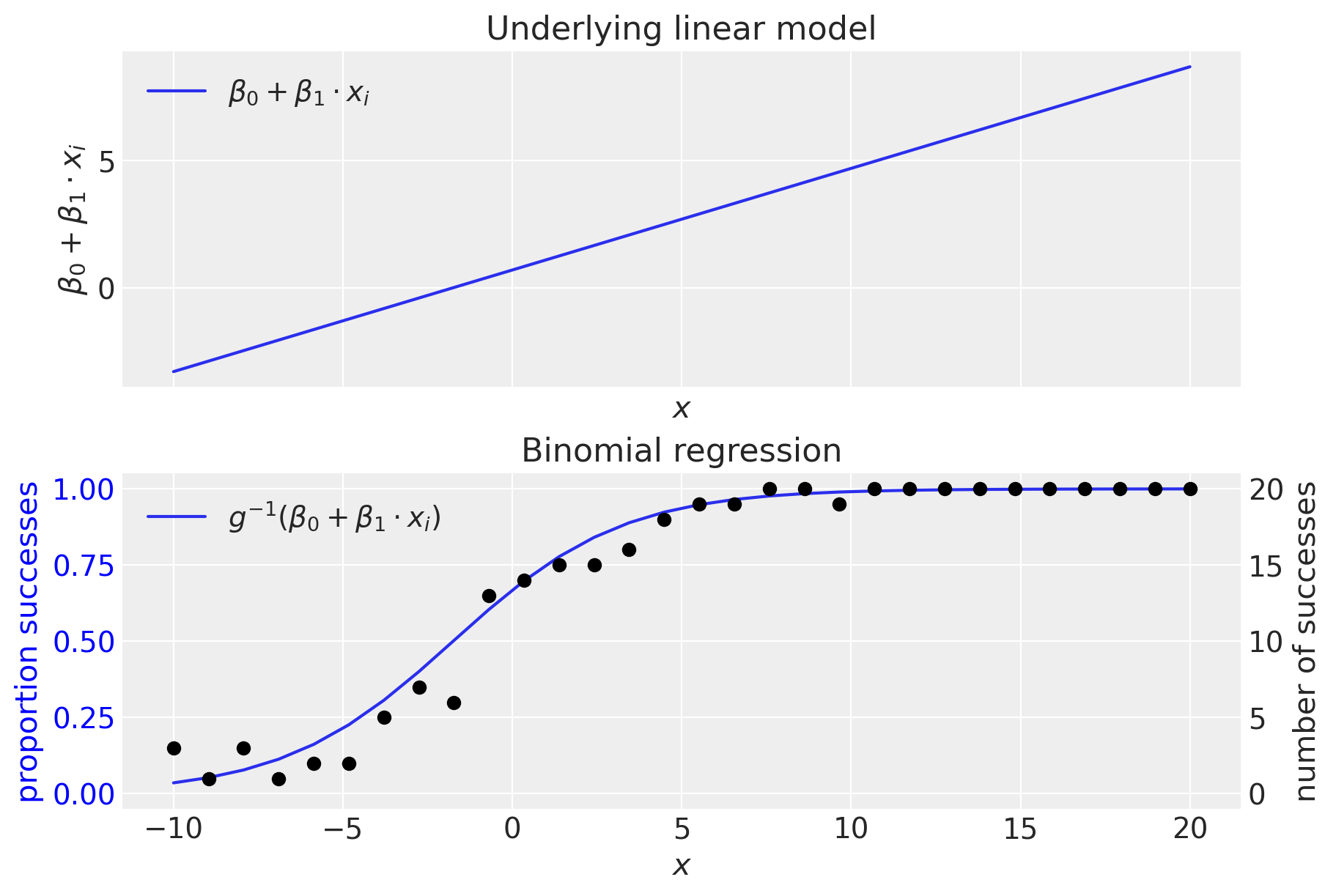
顶部面板显示了(未转换的)线性模型。我们可以看到,线性模型生成的值超出了范围 \(0-1\),这清楚地表明需要一个逆链接函数,\(g^{-1}()\),它将值从 \((-\infty, +\infty)\) 域转换到 \((0, 1)\) 域。正如我们所见,这是通过逆逻辑函数(也称为逻辑S形函数)完成的。
二项回归模型#
从技术上讲,我们不需要提供coords,但在后续重塑数据数组时,提供这个(观察值列表)会有所帮助。coords中的信息被模型中的dims关键字参数使用。
coords = {"observation": data.index.values}

with pm.Model(coords=coords) as binomial_regression_model:
    x = pm.ConstantData("x", data["x"], dims="observation")
    # priors
    beta0 = pm.Normal("beta0", mu=0, sigma=1)
    beta1 = pm.Normal("beta1", mu=0, sigma=1)
    # linear model
    mu = beta0 + beta1 * x
    p = pm.Deterministic("p", pm.math.invlogit(mu), dims="observation")
    # likelihood
    pm.Binomial("y", n=n, p=p, observed=data["y"], dims="observation")
pm.model_to_graphviz(binomial_regression_model)

with binomial_regression_model:
    idata = pm.sample(1000, tune=2000)
Sampling 4 chains for 2_000 tune and 1_000 draw iterations (8_000 + 4_000 draws total) took 1 seconds.
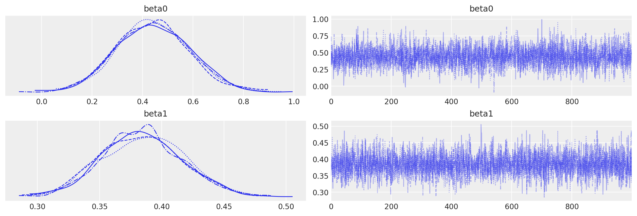
通过链的可视化检查确认没有推断问题。我们没有收到关于分歧、\(\hat{R}\)或有效样本量的警告。一切看起来都很好。
az.plot_trace(idata, var_names=["beta0", "beta1"]);
检查结果#
下面的代码在数据空间中绘制出模型预测,并在参数空间中展示我们的后验信念。
Show code cell source
fig, ax = plt.subplots(1, 2, figsize=(9, 4), gridspec_kw={"width_ratios": [2, 1]})

# Data space plot ========================================================
az.plot_hdi(
    data["x"],
    idata.posterior.p,
    hdi_prob=0.95,
    fill_kwargs={"alpha": 0.25, "linewidth": 0},
    ax=ax[0],
    color="C1",
)
# posterior mean
post_mean = idata.posterior.p.mean(("chain", "draw"))
ax[0].plot(data["x"], post_mean, label="posterior mean", color="C1")
# plot truth
ax[0].plot(data["x"], p_true, "--", label="true", color="C2")
# formatting
ax[0].set(xlabel="x", title="Data space")
ax[0].set_ylabel("proportion successes", color="C1")
ax[0].tick_params(axis="y", labelcolor="C1")
ax[0].legend()
# instantiate a second axes that shares the same x-axis
freq = ax[0].twinx()
freq.set_ylabel("number of successes")
freq.scatter(data["x"], data["y"], color="k", label="data")
# get y-axes to line up
y_buffer = 1
freq.set(ylim=[-y_buffer, n + y_buffer])
ax[0].set(ylim=[-(y_buffer / n), 1 + (y_buffer / n)])
freq.grid(None)
# set both y-axis to have 5 ticks
ax[0].set(yticks=np.linspace(0, 20, 5) / n)
freq.set(yticks=np.linspace(0, 20, 5))

# Parameter space plot ===================================================
az.plot_kde(
    az.extract(idata, var_names="beta0"),
    az.extract(idata, var_names="beta1"),
    contourf_kwargs={"cmap": "Blues"},
    ax=ax[1],
)
ax[1].plot(beta0_true, beta1_true, "C2o", label="true")
ax[1].set(xlabel=r"$\beta_0$", ylabel=r"$\beta_1$", title="Parameter space")
ax[1].legend(facecolor="white", frameon=True);
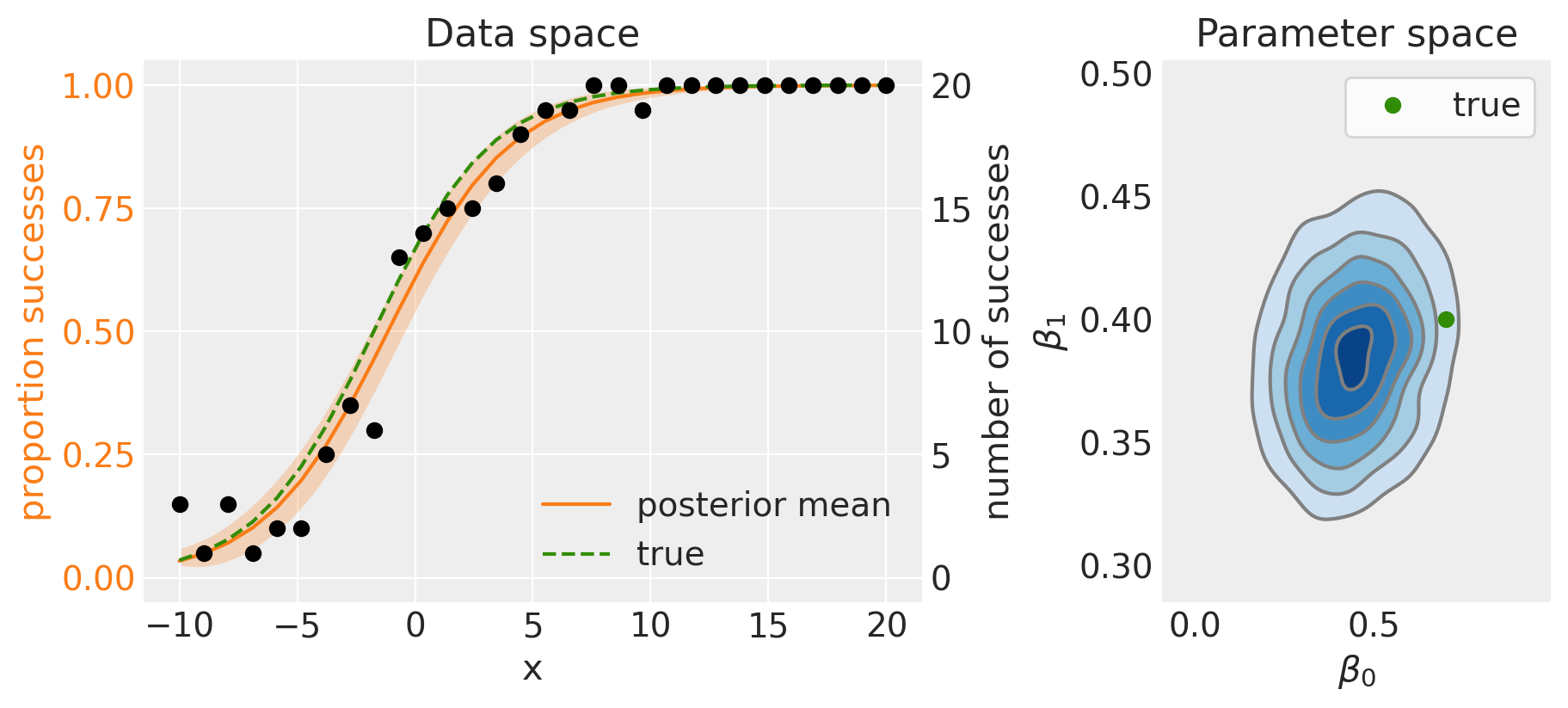
左侧面板显示了后验均值(实线)和95%可信区间(阴影区域)。由于我们使用的是模拟数据,我们知道真实模型是什么,因此可以看到后验均值与真实数据生成模型相比表现良好。
后验分布在参数空间中的表现(右侧面板)也很好地反映了这一点,与真实数据生成参数的比较效果良好。
在实际数据分析情况下使用二项回归可能涉及更多的预测变量和相应的更多模型参数,但希望这个例子已经展示了二项回归背后的逻辑。
参考资料#
Roback, P. 和 J. Legler. 超越多元线性回归:在R中应用广义线性模型和多层次模型. CRC出版社, 2021. URL: https://bookdown.org/roback/bookdown-BeyondMLR/.
水印#
%load_ext watermark
%watermark -n -u -v -iv -w -p pytensor,aeppl
Last updated: Sun Feb 05 2023

Python implementation: CPython
Python version       : 3.10.9
IPython version      : 8.9.0

pytensor: 2.8.11
aeppl   : not installed

matplotlib: 3.6.3
numpy     : 1.24.1
arviz     : 0.14.0
pandas    : 1.5.3
pymc      : 5.0.1

Watermark: 2.3.1