


GLM: 泊松回归#
这是一个使用虚拟数据预测计数的泊松回归的最小可重复示例。
这个笔记本主要是为了演示如何使用PyMC进行泊松回归,包括手动实现和使用bambi来演示使用formulae库的交互作用。我们将创建一些虚拟数据,这些数据根据线性模型泊松分布,并尝试通过推理恢复该线性模型的系数。
更多统计细节请参见:
关于Wikipedia的基本信息
广义线性模型:泊松回归、暴露和过度离散在ARM, Gelmann & Hill 2006的第6.2章中讨论。
这是来自ARM 6.2的工作示例,作者是Clay Ford
这个非常基础的模型是受到Ian Osvald 的一个项目的启发,该项目旨在理解外部环境因素对测试对象过敏性打喷嚏的各种影响。
#!pip install seaborn
import arviz as az
import bambi as bmb
import matplotlib.pyplot as plt
import numpy as np
import pandas as pd
import pymc as pm
import seaborn as sns

from formulae import design_matrices
RANDOM_SEED = 8927
rng = np.random.default_rng(RANDOM_SEED)

%config InlineBackend.figure_format = 'retina'
az.style.use("arviz-darkgrid")
局部函数#
生成数据#
这个虚拟数据集是为了模拟一项关于量化自我研究的某些数据而创建的,实际数据比这个更复杂。如果你想知道更多,可以问Ian Osvald @ianozvald。
假设:#
该主题每天打喷嚏N次,记录为
nsneeze (int)受试者在那一天可能饮酒也可能不饮酒,记录为
alcohol (布尔值)受试者在那一天可能服用也可能不服用抗组胺药物,记录为负向行为
nomeds (布尔值)我们假设(可能不正确)打喷嚏以某种基线频率发生,如果不服用抗组胺药,频率会增加,并且在饮酒后进一步增加。
数据按天汇总,以得出当天打喷嚏的总次数,并带有酒精和抗组胺药使用的布尔标志,其大前提是打喷嚏次数与这些因素有直接的因果关系。
创建4000天的数据:每天的喷嚏次数,这些次数是关于酒精消耗和抗组胺药使用的泊松分布
# decide poisson theta values
theta_noalcohol_meds = 1  # no alcohol, took an antihist
theta_alcohol_meds = 3  # alcohol, took an antihist
theta_noalcohol_nomeds = 6  # no alcohol, no antihist
theta_alcohol_nomeds = 36  # alcohol, no antihist

# create samples
q = 1000
df = pd.DataFrame(
    {
        "nsneeze": np.concatenate(
            (
                rng.poisson(theta_noalcohol_meds, q),
                rng.poisson(theta_alcohol_meds, q),
                rng.poisson(theta_noalcohol_nomeds, q),
                rng.poisson(theta_alcohol_nomeds, q),
            )
        ),
        "alcohol": np.concatenate(
            (
                np.repeat(False, q),
                np.repeat(True, q),
                np.repeat(False, q),
                np.repeat(True, q),
            )
        ),
        "nomeds": np.concatenate(
            (
                np.repeat(False, q),
                np.repeat(False, q),
                np.repeat(True, q),
                np.repeat(True, q),
            )
        ),
    }
)
df.tail()
| nsneeze | alcohol | nomeds | |
|---|---|---|---|
| 3995 | 26 | True | True |
| 3996 | 35 | True | True |
| 3997 | 36 | True | True |
| 3998 | 32 | True | True |
| 3999 | 35 | True | True |
查看各种组合的均值(泊松均值)#
df.groupby(["alcohol", "nomeds"]).mean().unstack()
| nsneeze | ||
|---|---|---|
| nomeds | False | True |
| alcohol | ||
| False | 1.047 | 5.981 |
| True | 2.986 | 35.929 |
简要描述数据集#
g = sns.catplot(
    x="nsneeze",
    row="nomeds",
    col="alcohol",
    data=df,
    kind="count",
    height=4,
    aspect=1.5,
)
for ax in (g.axes[1, 0], g.axes[1, 1]):
    for n, label in enumerate(ax.xaxis.get_ticklabels()):
        label.set_visible(n % 5 == 0)
/Users/reshamashaikh/miniforge3/envs/pymc-ex/lib/python3.10/site-packages/seaborn/axisgrid.py:118: UserWarning: This figure was using constrained_layout, but that is incompatible with subplots_adjust and/or tight_layout; disabling constrained_layout.
  self._figure.tight_layout(*args, **kwargs)
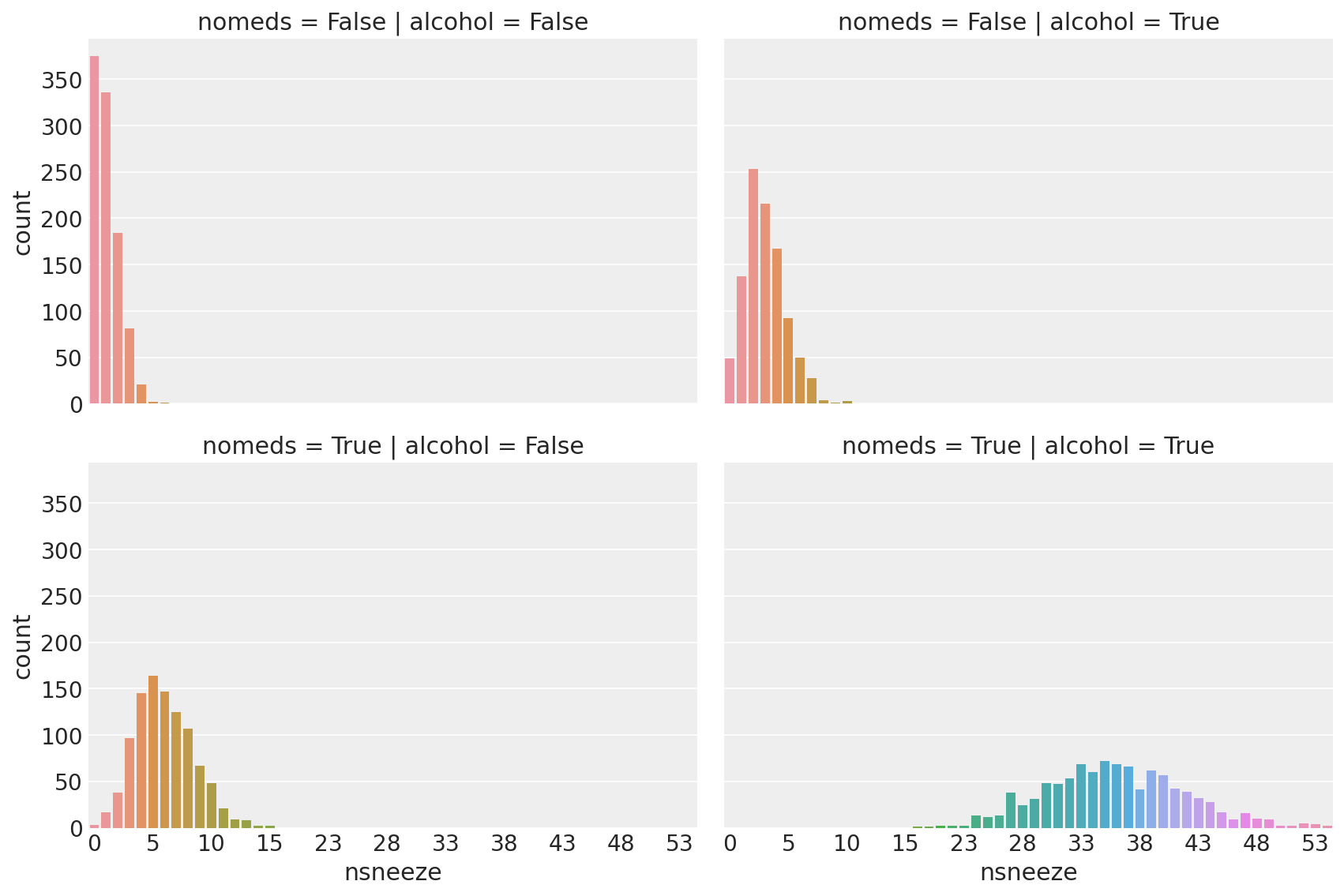
观察:
这看起来很像泊松分布的计数数据(因为它是)
当
nomeds == False且alcohol == False时(左上角,即使用了抗组胺药,但没有饮酒),打喷嚏次数的泊松分布的均值较低。将
alcohol == True(右上角)更改为会增加打喷嚏次数nsneeze略微增加更改
nomeds == True(左下角)会进一步增加打喷嚏次数nsneeze同时改变
alcohol == True and nomeds == True(右下角)会大大增加打喷嚏次数nsneeze,增加均值和方差。
泊松回归#
我们的模型是一个非常简单的泊松回归,允许项之间的交互:
创建用于项交互的线性模型
fml = "nsneeze ~ alcohol + nomeds + alcohol:nomeds" # full formulae formulation
fml = "nsneeze ~ alcohol * nomeds" # lazy, alternative formulae formulation
1. 手动方法,创建设计矩阵并手动指定模型#
创建设计矩阵
dm = design_matrices(fml, df, na_action="error")
mx_ex = dm.common.as_dataframe()
mx_en = dm.response.as_dataframe()
mx_ex
| Intercept | alcohol | nomeds | alcohol:nomeds | |
|---|---|---|---|---|
| 0 | 1 | 0 | 0 | 0 |
| 1 | 1 | 0 | 0 | 0 |
| 2 | 1 | 0 | 0 | 0 |
| 3 | 1 | 0 | 0 | 0 |
| 4 | 1 | 0 | 0 | 0 |
| ... | ... | ... | ... | ... |
| 3995 | 1 | 1 | 1 | 1 |
| 3996 | 1 | 1 | 1 | 1 |
| 3997 | 1 | 1 | 1 | 1 |
| 3998 | 1 | 1 | 1 | 1 |
| 3999 | 1 | 1 | 1 | 1 |
4000行 × 4列
创建模型
with pm.Model() as mdl_fish:
    # define priors, weakly informative Normal
    b0 = pm.Normal("Intercept", mu=0, sigma=10)
    b1 = pm.Normal("alcohol", mu=0, sigma=10)
    b2 = pm.Normal("nomeds", mu=0, sigma=10)
    b3 = pm.Normal("alcohol:nomeds", mu=0, sigma=10)

    # define linear model and exp link function
    theta = (
        b0
        + b1 * mx_ex["alcohol"].values
        + b2 * mx_ex["nomeds"].values
        + b3 * mx_ex["alcohol:nomeds"].values
    )

    ## Define Poisson likelihood
    y = pm.Poisson("y", mu=pm.math.exp(theta), observed=mx_en["nsneeze"].values)
示例模型
with mdl_fish:
    inf_fish = pm.sample()
    # inf_fish.extend(pm.sample_posterior_predictive(inf_fish))
Auto-assigning NUTS sampler...
Initializing NUTS using jitter+adapt_diag...
Multiprocess sampling (2 chains in 2 jobs)
NUTS: [Intercept, alcohol, nomeds, alcohol:nomeds]
Sampling 2 chains for 1_000 tune and 1_000 draw iterations (2_000 + 2_000 draws total) took 36 seconds.
查看诊断
az.plot_trace(inf_fish);
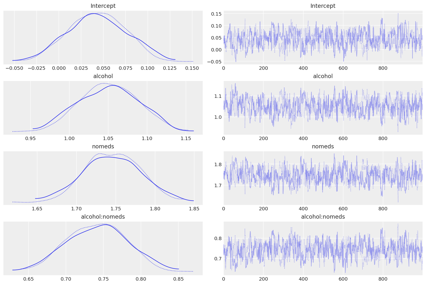
观察:
模型收敛迅速,轨迹图看起来混合得很好
转换系数并恢复theta值#
az.summary(np.exp(inf_fish.posterior), kind="stats")
| mean | sd | hdi_3% | hdi_97% | |
|---|---|---|---|---|
| Intercept | 1.045 | 0.034 | 0.981 | 1.106 |
| alcohol | 2.862 | 0.109 | 2.668 | 3.065 |
| nomeds | 5.734 | 0.205 | 5.341 | 6.115 |
| alcohol:nomeds | 2.102 | 0.086 | 1.948 | 2.266 |
观察:
每个特征对基准打喷嚏次数的乘数贡献似乎如数据生成所示:
exp(截距): 均值=1.05 cr=[0.98, 1.10]
大致线性基线计数,当没有酒精和药物时,根据生成的数据:
theta_noalcohol_meds = 1(如上所设) theta_noalcohol_meds = exp(截距) = 1
exp(alcohol): 均值=2.86 置信区间=[2.67, 3.07]
添加酒精的非零正面效果,根据生成的数据,是基准打喷嚏次数的约3倍乘数:
theta_alcohol_meds = 3 (如上所设) theta_alcohol_meds = exp(截距 + 酒精) = exp(截距) * exp(酒精) = 1 * 3 = 3
exp(nomeds): 平均值=5.73 置信区间=[5.34, 6.08]
添加nomeds的较大、非零的正面效果,生成的数据显示,这是基准喷嚏次数的约6倍乘数:
theta_noalcohol_nomeds = 6(如上所设) theta_noalcohol_nomeds = exp(Intercept + nomeds) = exp(Intercept) * exp(nomeds) = 1 * 6 = 6
exp(alcohol:nomeds): 平均值=2.10 置信区间=[1.96, 2.28]
酒精和药物的小幅正面交互作用,根据生成的数据,是基础喷嚏次数的约2倍乘数:
theta_alcohol_nomeds = 36(如上所设) theta_alcohol_nomeds = exp(截距 + 酒精 + 无药物 + 酒精:无药物) = exp(截距) * exp(酒精) * exp(无药物 * 酒精:无药物) = 1 * 3 * 6 * 2 = 36
2. 替代方法,使用 bambi#
创建模型
使用bambi的替代自动公式
model = bmb.Model(fml, df, family="poisson")
拟合模型
inf_fish_alt = model.fit()
Auto-assigning NUTS sampler...
Initializing NUTS using jitter+adapt_diag...
Multiprocess sampling (2 chains in 2 jobs)
NUTS: [Intercept, alcohol, nomeds, alcohol:nomeds]
Sampling 2 chains for 1_000 tune and 1_000 draw iterations (2_000 + 2_000 draws total) took 36 seconds.
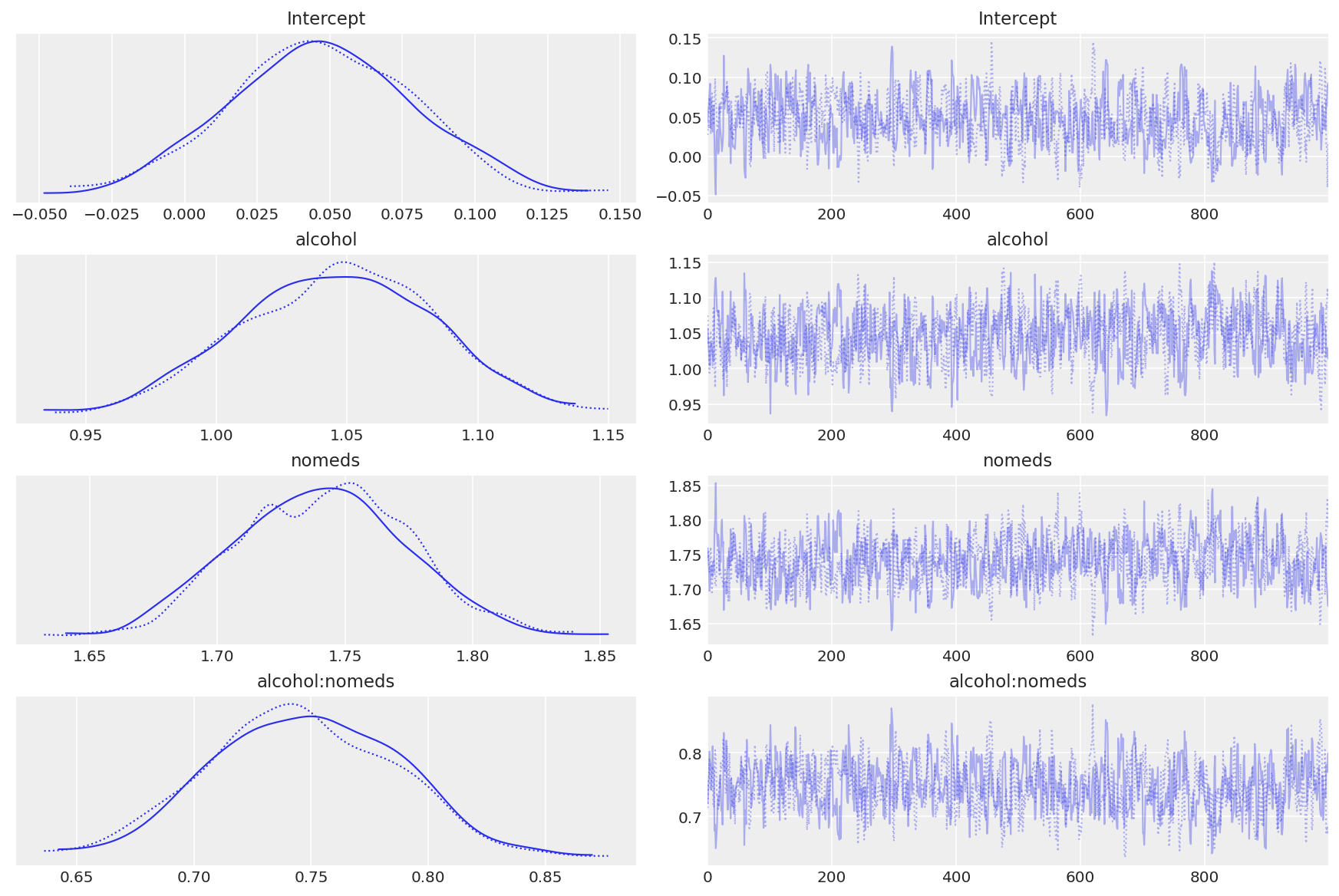
查看跟踪
az.plot_trace(inf_fish_alt);
转换系数#
az.summary(np.exp(inf_fish_alt.posterior), kind="stats")
| mean | sd | hdi_3% | hdi_97% | |
|---|---|---|---|---|
| Intercept | 1.049 | 0.033 | 0.987 | 1.107 |
| alcohol | 2.849 | 0.105 | 2.659 | 3.047 |
| nomeds | 5.708 | 0.190 | 5.362 | 6.058 |
| alcohol:nomeds | 2.111 | 0.083 | 1.960 | 2.258 |
观察:
轨迹图看起来混合良好
转换后的模型系数看起来与手动模型生成的系数大致相同
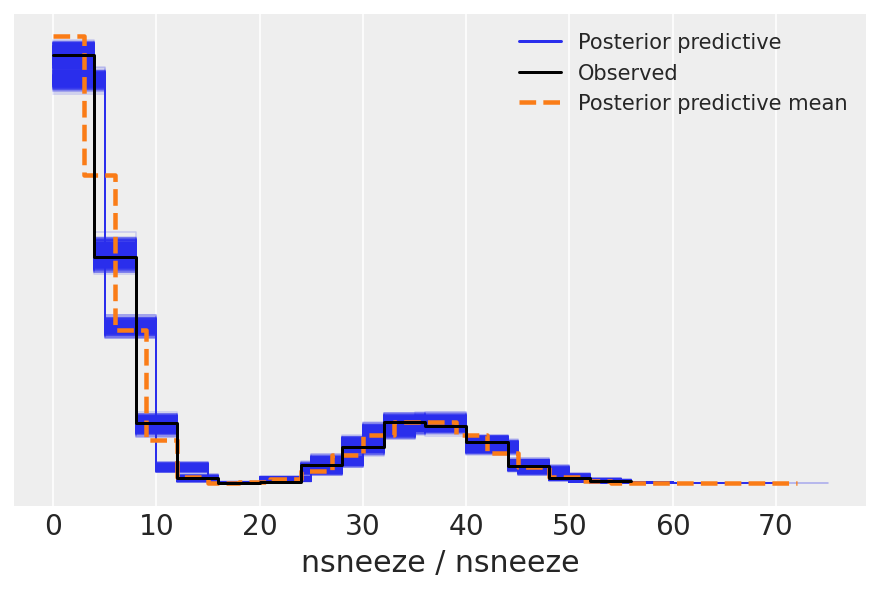
请注意,后验预测样本具有极端偏斜
posterior_predictive = model.predict(inf_fish_alt, kind="pps")
我们可以使用 az.plot_ppc() 来检查后验预测样本是否与观测数据相似。
有关后验预测检查的更多信息,我们可以参考先验和后验预测检查。
az.plot_ppc(inf_fish_alt);
水印#
%load_ext watermark
%watermark -n -u -v -iv -w -p pytensor,aeppl
Last updated: Wed Nov 30 2022

Python implementation: CPython
Python version       : 3.10.5
IPython version      : 8.4.0

pytensor: 2.7.5
aeppl : 0.0.32

matplotlib: 3.5.2
seaborn   : 0.12.1
pymc      : 4.1.2
numpy     : 1.21.6
pandas    : 1.4.3
arviz     : 0.12.1
bambi     : 0.9.1

Watermark: 2.3.1