


贝叶斯缺失数据插补#
import random

import arviz as az
import matplotlib.cm as cm
import matplotlib.pyplot as plt
import numpy as np
import pandas as pd
import pymc as pm
import scipy.optimize

from matplotlib.lines import Line2D
from pymc.sampling.jax import sample_blackjax_nuts, sample_numpyro_nuts
from scipy.stats import multivariate_normal
/Users/nathanielforde/opt/miniconda3/envs/missing_data_clean/lib/python3.11/site-packages/pymc/sampling/jax.py:39: UserWarning: This module is experimental.
  warnings.warn("This module is experimental.")
贝叶斯插补与缺失程度#
缺失值数据的分析是因果推断研究的一个入口。
任何受缺失数据困扰的分析的关键特征之一是支配缺失性质的假设,即我们的数据中存在缺口的原因是什么?我们可以忽略它们吗?我们应该担心为什么吗?在本笔记本中,我们将看到一个如何使用最大似然估计和贝叶斯插补技术处理缺失数据的示例。这将引发关于在存在缺失数据的情况下支配推断的假设,以及在反事实情况下的推断的问题。
我们将通过一个员工满意度调查的示例分析来具体讨论,并探讨不同的工作条件如何影响我们在数据中看到的回答和未回答的情况。
%config InlineBackend.figure_format = 'retina'  # high resolution figures
az.style.use("arviz-darkgrid")
rng = np.random.default_rng(42)
缺失数据分类#
鲁宾的著名分类法将问题分解为三个基本选项的选择:
完全随机缺失 (MCAR)
随机缺失 (MAR)
缺失非随机 (MNAR)
这些范式中的每一个都可以简化为关于缺失数据模式的条件概率的明确定义。第一种模式是最不令人担忧的。(MCAR)假设指出,数据缺失的方式与已实现数据的观察部分和未观察部分都无关。它缺失是由于世界的偶然情况 \(\phi\)。
而第二种模式(MAR)允许缺失的原因可以是观察数据和世界环境的函数。有时这被称为可忽略缺失的情况,因为可以根据观察到的数据进行良好的估计。可能会有精度损失,但推论应该是正确的。
最恶劣的缺失数据类型是当缺失性是观测数据之外的某个因素的函数,并且该方程无法进一步简化时。在这种情况下,由于混杂的风险,填补和估计的努力可能会变得更加困难。这是一种不可忽略的缺失性情况。
这些假设在任何分析开始之前就已经做出。它们本质上是不可验证的。你的分析是否成立取决于每个假设在你试图应用它们的情境中是否合理。例如,另一种类型的缺失数据是由于系统性审查导致的,如在贝叶斯回归与截断或审查数据中所讨论的。在这种情况下,审查的原因决定了缺失的模式。
员工满意度调查#
我们将遵循Craig Enders的《应用缺失数据分析》Enders K [2022]的介绍,并使用员工满意度数据集进行工作。该数据集包括一些报告员工工作条件和满意度的综合指标。特别值得注意的是授权(empower)、工作满意度(worksat)以及两个综合调查分数,记录了员工的领导力气候(climate)和与主管的关系质量(lmx)。
关键问题是哪些假设支配了我们缺失数据的模式。
try:
    df_employee = pd.read_csv("../data/employee.csv")
except FileNotFoundError:
    df_employee = pd.read_csv(pm.get_data("employee.csv"))
df_employee.head()
| employee | team | turnover | male | empower | lmx | worksat | climate | cohesion | |
|---|---|---|---|---|---|---|---|---|---|
| 0 | 1 | 1 | 0.0 | 1 | 32.0 | 11.0 | 3.0 | 18.0 | 3.5 |
| 1 | 2 | 1 | 1.0 | 1 | NaN | 13.0 | 4.0 | 18.0 | 3.5 |
| 2 | 3 | 1 | 1.0 | 1 | 30.0 | 9.0 | 4.0 | 18.0 | 3.5 |
| 3 | 4 | 1 | 1.0 | 1 | 29.0 | 8.0 | 3.0 | 18.0 | 3.5 |
| 4 | 5 | 1 | 1.0 | 0 | 26.0 | 7.0 | 4.0 | 18.0 | 3.5 |
# Percentage Missing
df_employee[["worksat", "empower", "lmx"]].isna().sum() / len(df_employee)
worksat    0.047619
empower    0.161905
lmx        0.041270
dtype: float64
# Patterns of missing Data
df_employee[["worksat", "empower", "lmx"]].isnull().drop_duplicates().reset_index(drop=True)
| worksat | empower | lmx | |
|---|---|---|---|
| 0 | False | False | False |
| 1 | False | True | False |
| 2 | True | True | False |
| 3 | False | False | True |
| 4 | True | False | False |
fig, ax = plt.subplots(figsize=(20, 7))
ax.hist(df_employee["empower"], bins=30, ec="black", color="cyan", label="Empowerment")
ax.hist(df_employee["lmx"], bins=30, ec="black", color="yellow", label="LMX")
ax.hist(df_employee["worksat"], bins=30, ec="black", color="green", label="Work Satisfaction")
ax.set_title("Employee Satisfaction Survey Results", fontsize=20)
ax.legend();
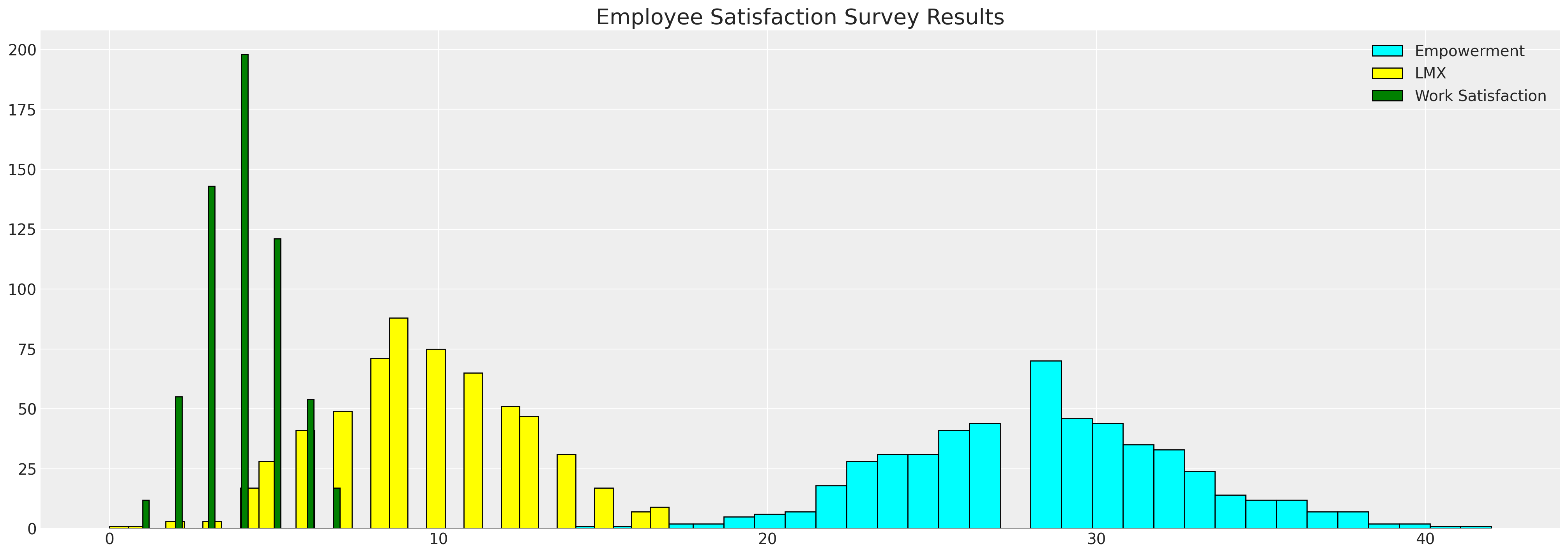
我们在这里看到的是员工指标的直方图。我们希望通过填补数据中的空白来更好地理解变量之间的关系,以及一个变量中的空白如何可能由其他变量的值所驱动。
FIML: 全信息最大似然法#
这种处理缺失数据的方法不是插补方法。它使用最大似然估计来估计多元正态分布的参数,这些参数最能生成我们观察到的数据。与直接的最大似然估计方法相比,这种方法稍微复杂一些,因为它尊重我们原始数据集中存在缺失数据的事实,但基本思想是相同的。我们希望优化多元正态分布的参数,以最好地拟合观察到的数据。
该过程通过将数据划分为其“缺失性”模式,并将每个分区视为对我们要最大化的最终对数似然项的贡献。我们将它们的贡献结合起来,以估计多元正态分布的拟合。
data = df_employee[["worksat", "empower", "lmx"]]


def split_data_by_missing_pattern(data):
    # We want to extract our the pattern of missing-ness in our dataset
    # and save each sub-set of our data in a structure that can be used to feed into a log-likelihood function
    grouped_patterns = []
    patterns = data.notnull().drop_duplicates().values
    # A pattern is whether the values in each column e.g. [True, True, True] or [True, True, False]
    observed = data.notnull()
    for p in range(len(patterns)):
        temp = observed[
            (observed["worksat"] == patterns[p][0])
            & (observed["empower"] == patterns[p][1])
            & (observed["lmx"] == patterns[p][2])
        ]
        grouped_patterns.append([patterns[p], temp.index, data.iloc[temp.index].dropna(axis=1)])

    return grouped_patterns


def reconstitute_params(params_vector, n_vars):
    # Convenience numpy function to construct mirrored COV matrix
    # From flattened params_vector
    mus = params_vector[0:n_vars]
    cov_flat = params_vector[n_vars:]
    indices = np.tril_indices(n_vars)
    cov = np.empty((n_vars, n_vars))
    for i, j, c in zip(indices[0], indices[1], cov_flat):
        cov[i, j] = c
        cov[j, i] = c
    cov = cov + 1e-25
    return mus, cov


def optimise_ll(flat_params, n_vars, grouped_patterns):
    mus, cov = reconstitute_params(flat_params, n_vars)
    # Check if COV is positive definite
    if (np.linalg.eigvalsh(cov) < 0).any():
        return 1e100
    objval = 0.0
    for obs_pattern, _, obs_data in grouped_patterns:
        # This is the key (tricky) step because we're selecting the variables which pattern
        # the full information set within each pattern of "missing-ness"
        # e.g. when the observed pattern is [True, True, False] we want the first two variables
        # of the mus vector and we want only the covariance relations between the relevant variables from the cov
        # in the iteration.
        obs_mus = mus[obs_pattern]
        obs_cov = cov[obs_pattern][:, obs_pattern]
        ll = np.sum(multivariate_normal(obs_mus, obs_cov).logpdf(obs_data))
        objval = ll + objval
    return -objval


def estimate(data):
    n_vars = data.shape[1]
    # Initialise
    mus0 = np.zeros(n_vars)
    cov0 = np.eye(n_vars)
    # Flatten params for optimiser
    params0 = np.append(mus0, cov0[np.tril_indices(n_vars)])
    # Process Data
    grouped_patterns = split_data_by_missing_pattern(data)
    # Run the Optimiser.
    try:
        result = scipy.optimize.minimize(
            optimise_ll, params0, args=(n_vars, grouped_patterns), method="Powell"
        )
    except Exception as e:
        raise e
    mean, cov = reconstitute_params(result.x, n_vars)
    return mean, cov


fiml_mus, fiml_cov = estimate(data)


print("Full information Maximum Likelihood Estimate Mu:")
display(pd.DataFrame(fiml_mus, index=data.columns).T)
print("Full information Maximum Likelihood Estimate COV:")
pd.DataFrame(fiml_cov, columns=data.columns, index=data.columns)
Full information Maximum Likelihood Estimate Mu:
| worksat | empower | lmx | |
|---|---|---|---|
| 0 | 3.983351 | 28.595211 | 9.624485 |
Full information Maximum Likelihood Estimate COV:
| worksat | empower | lmx | |
|---|---|---|---|
| worksat | 1.568676 | 1.599817 | 1.547433 |
| empower | 1.599817 | 19.138522 | 5.428954 |
| lmx | 1.547433 | 5.428954 | 8.934030 |
从隐含分布中采样#
然后我们可以从隐含的分布中进行采样,以估计其他感兴趣的特征,并根据观测数据进行测试。
mle_fit = multivariate_normal(fiml_mus, fiml_cov)
mle_sample = mle_fit.rvs(10000)
mle_sample = pd.DataFrame(mle_sample, columns=["worksat", "empower", "lmx"])
mle_sample.head()
| worksat | empower | lmx | |
|---|---|---|---|
| 0 | 4.467296 | 31.568011 | 12.418765 |
| 1 | 4.713191 | 30.329419 | 10.651786 |
| 2 | 5.699765 | 35.770312 | 12.558135 |
| 3 | 4.067691 | 27.874578 | 6.271341 |
| 4 | 3.580109 | 28.799105 | 9.704713 |
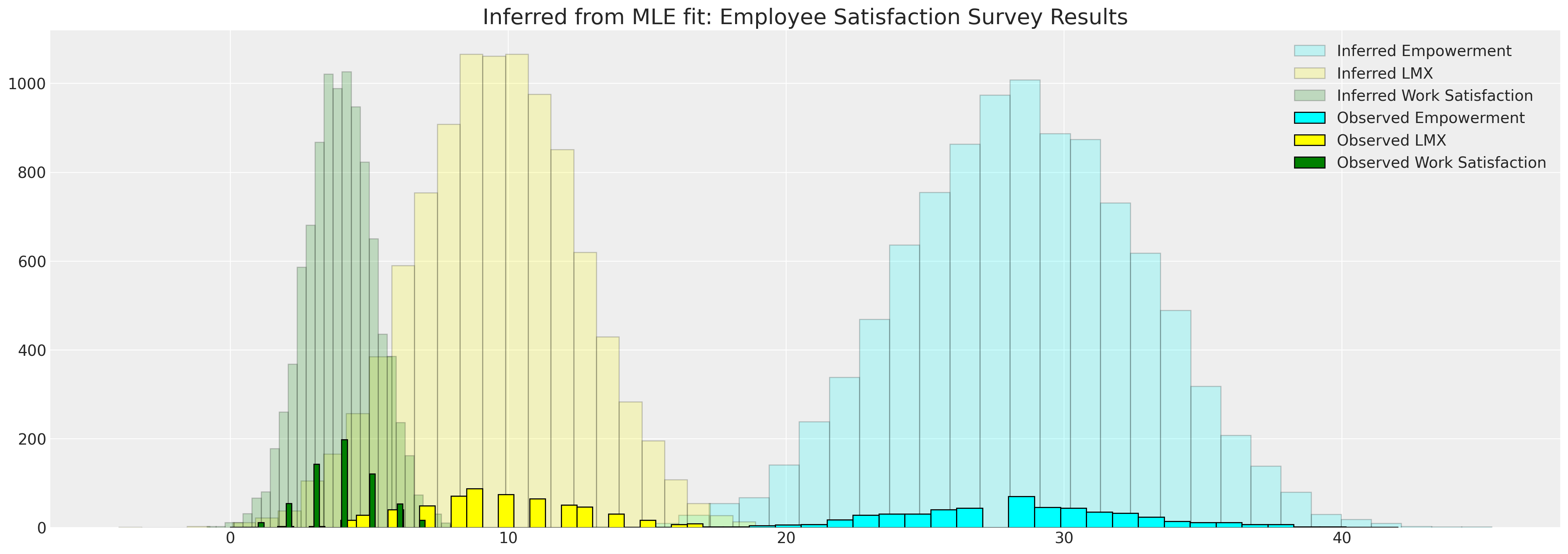
这使我们能够将隐含分布与观测数据进行比较
fig, ax = plt.subplots(figsize=(20, 7))
ax.hist(
    mle_sample["empower"],
    bins=30,
    ec="black",
    color="cyan",
    alpha=0.2,
    label="Inferred Empowerment",
)
ax.hist(mle_sample["lmx"], bins=30, ec="black", color="yellow", alpha=0.2, label="Inferred LMX")
ax.hist(
    mle_sample["worksat"],
    bins=30,
    ec="black",
    color="green",
    alpha=0.2,
    label="Inferred Work Satisfaction",
)
ax.hist(data["empower"], bins=30, ec="black", color="cyan", label="Observed Empowerment")
ax.hist(data["lmx"], bins=30, ec="black", color="yellow", label="Observed LMX")
ax.hist(data["worksat"], bins=30, ec="black", color="green", label="Observed Work Satisfaction")
ax.set_title("Inferred from MLE fit: Employee Satisfaction Survey Results", fontsize=20)
ax.legend()
<matplotlib.legend.Legend at 0x1914bce50>
插补指标数据之间的相关性#
我们还可以从样本中计算其他感兴趣的特征。例如,我们可能想知道所讨论变量之间的相关性。
pd.DataFrame(mle_sample.corr(), columns=data.columns, index=data.columns)
| worksat | empower | lmx | |
|---|---|---|---|
| worksat | 1.000000 | 0.300790 | 0.409996 |
| empower | 0.300790 | 1.000000 | 0.410874 |
| lmx | 0.409996 | 0.410874 | 1.000000 |
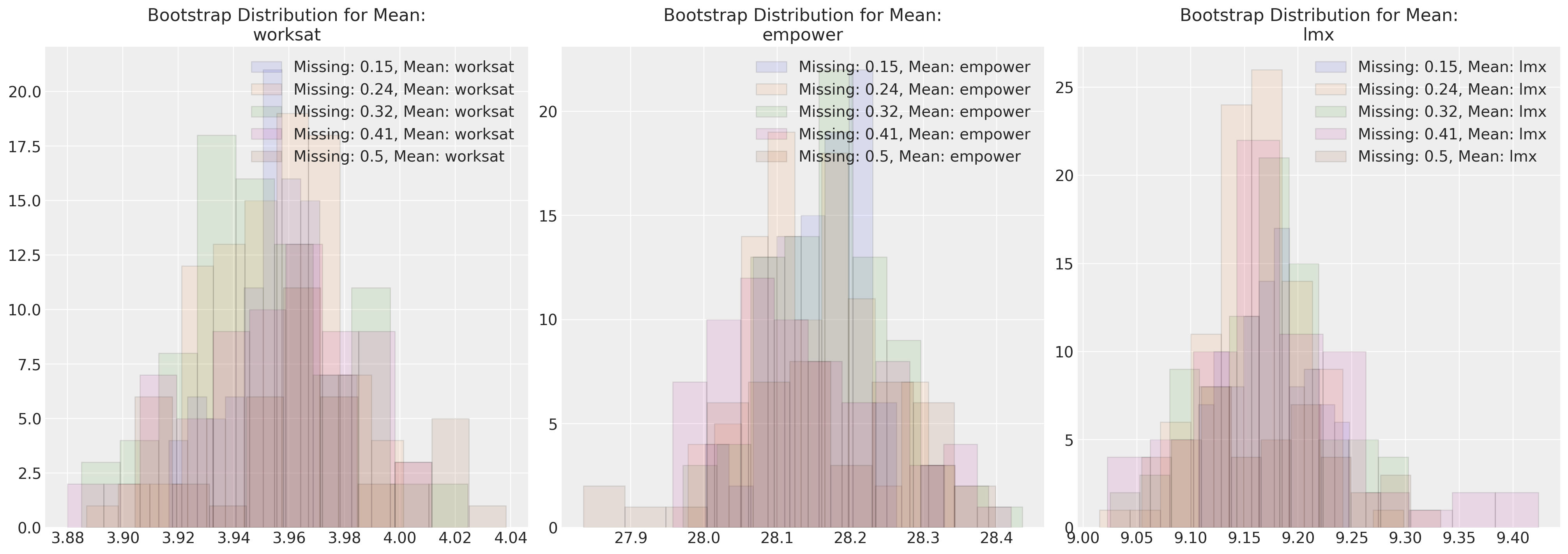
自举敏感性分析#
我们可能还希望在不同缺失性规范下,将估计的参数与自举样本进行验证。
data_200 = df_employee[["worksat", "empower", "lmx"]].dropna().sample(200)
data_200.reset_index(inplace=True, drop=True)


sensitivity = {}
n_missing = np.linspace(30, 100, 5)  # Change or alter the range as desired
bootstrap_iterations = 100  # change to large number running a real analysis in this case
for n in n_missing:
    sensitivity[int(n)] = {}
    sensitivity[int(n)]["mus"] = []
    sensitivity[int(n)]["cov"] = []
    for i in range(bootstrap_iterations):
        temp = data_200.copy()
        for m in range(int(n)):
            i = random.choice(range(200))
            j = random.choice(range(3))
            temp.iloc[i, j] = np.nan
        try:
            fiml_mus, fiml_cov = estimate(temp)
            sensitivity[int(n)]["mus"].append(fiml_mus)
            sensitivity[int(n)]["cov"].append(fiml_cov)
        except Exception as e:
            next
在这里,我们将最大似然参数估计值与各种缺失数据情况进行对比。这种方法可以应用于任何插补方法。
fig, axs = plt.subplots(1, 3, figsize=(20, 7))
for n in sensitivity.keys():
    temp = pd.DataFrame(sensitivity[n]["mus"], columns=["worksat", "empower", "lmx"])
    for col, ax in zip(temp.columns, axs):
        ax.hist(
            temp[col], alpha=0.1, ec="black", label=f"Missing: {np.round(n/200, 2)}, Mean: {col}"
        )
        ax.legend()
        ax.set_title(f"Bootstrap Distribution for Mean:\n{col}")
fig, axs = plt.subplots(2, 3, figsize=(20, 14))
axs = axs.flatten()
for n in sensitivity.keys():
    length = len(sensitivity[n]["cov"])
    temp = pd.DataFrame(
        [sensitivity[n]["cov"][i][np.tril_indices(3)] for i in range(length)],
        columns=[
            "var(worksat)",
            "cov(worksat, empower)",
            "var(empower)",
            "cov(worksat, lmx)",
            "cov(lmx, empower)",
            "var(lmx)",
        ],
    )
    for col, ax in zip(temp.columns, axs):
        ax.hist(
            temp[col], alpha=0.1, ec="black", label=f"Missing: {np.round(n/200, 2)}, Mean: {col}"
        )
        ax.legend()
        ax.set_title(f"Bootstrap Distribution for Expected:\n{col}")
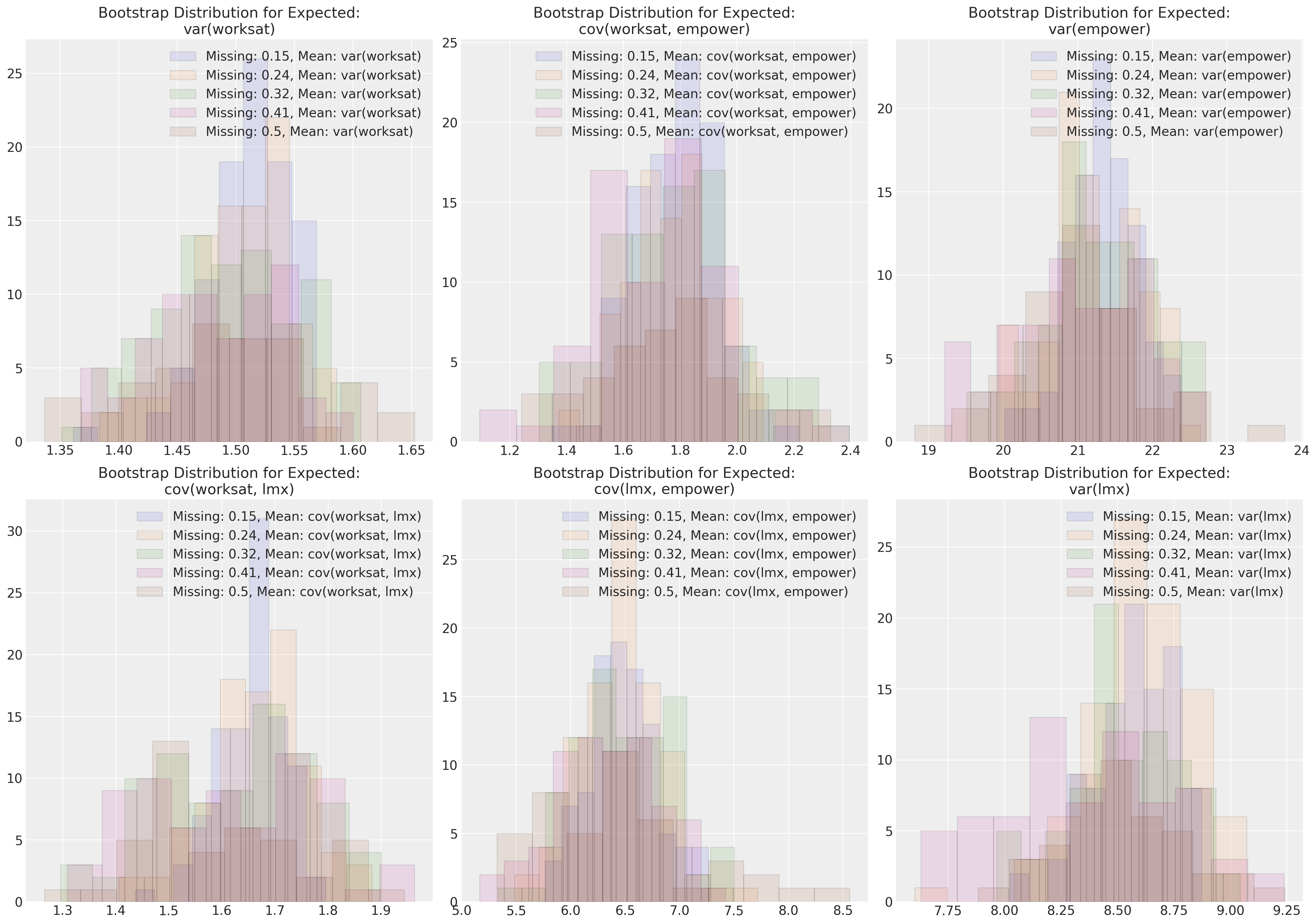
这些图表展示了在完全随机缺失(MCAR)情况下,我们的多元正态分布的参数估计对不同程度的缺失数据的鲁棒性。尝试在其他缺失数据机制下进行类似的模拟练习是一个有教育意义的练习。
贝叶斯插补#
接下来,我们将应用贝叶斯方法来解决相同的问题。但在这里,我们将使用后验预测分布直接填补缺失值。贝叶斯填补方法与我们之前看到的方法有所不同。我们不仅仅是在学习数据生成分布的参数(尽管我们也在这样做),贝叶斯过程通过MCMC采样直接为特定的缺失条目填补缺失值。
import pytensor.tensor as pt

with pm.Model() as model:
    # Priors
    mus = pm.Normal("mus", 0, 1, size=3)
    cov_flat_prior, _, _ = pm.LKJCholeskyCov("cov", n=3, eta=1.0, sd_dist=pm.Exponential.dist(1))
    # Create a vector of flat variables for the unobserved components of the MvNormal
    x_unobs = pm.Uniform("x_unobs", 0, 100, shape=(np.isnan(data.values).sum(),))

    # Create the symbolic value of x, combining observed data and unobserved variables
    x = pt.as_tensor(data.values)
    x = pm.Deterministic("x", pt.set_subtensor(x[np.isnan(data.values)], x_unobs))

    # Add a Potential with the logp of the variable conditioned on `x`
    pm.Potential("x_logp", pm.logp(rv=pm.MvNormal.dist(mus, chol=cov_flat_prior), value=x))
    idata = pm.sample_prior_predictive()
    idata = pm.sample()
    idata.extend(pm.sample(random_seed=120))
    pm.sample_posterior_predictive(idata, extend_inferencedata=True)

pm.model_to_graphviz(model)
/var/folders/99/gp2xl6x513s0tvl3cx79zf7m0000gn/T/ipykernel_96943/3865616598.py:16: UserWarning: The effect of Potentials on other parameters is ignored during prior predictive sampling. This is likely to lead to invalid or biased predictive samples.
  idata = pm.sample_prior_predictive()
Sampling: [cov, mus, x_unobs]
Auto-assigning NUTS sampler...
Initializing NUTS using jitter+adapt_diag...
Multiprocess sampling (4 chains in 4 jobs)
NUTS: [mus, cov, x_unobs]
/Users/nathanielforde/opt/miniconda3/envs/missing_data_clean/lib/python3.11/site-packages/pytensor/compile/function/types.py:972: RuntimeWarning: invalid value encountered in accumulate
  self.vm()
Sampling 4 chains for 1_000 tune and 1_000 draw iterations (4_000 + 4_000 draws total) took 98 seconds.
Auto-assigning NUTS sampler...
Initializing NUTS using jitter+adapt_diag...
Multiprocess sampling (4 chains in 4 jobs)
NUTS: [mus, cov, x_unobs]
/Users/nathanielforde/opt/miniconda3/envs/missing_data_clean/lib/python3.11/site-packages/pytensor/compile/function/types.py:972: RuntimeWarning: invalid value encountered in accumulate
  self.vm()
/Users/nathanielforde/opt/miniconda3/envs/missing_data_clean/lib/python3.11/site-packages/pytensor/compile/function/types.py:972: RuntimeWarning: invalid value encountered in accumulate
  self.vm()
Sampling 4 chains for 1_000 tune and 1_000 draw iterations (4_000 + 4_000 draws total) took 99 seconds.
/var/folders/99/gp2xl6x513s0tvl3cx79zf7m0000gn/T/ipykernel_96943/3865616598.py:19: UserWarning: The effect of Potentials on other parameters is ignored during posterior predictive sampling. This is likely to lead to invalid or biased predictive samples.
  pm.sample_posterior_predictive(idata, extend_inferencedata=True)

az.plot_posterior(idata, var_names=["mus", "cov"]);
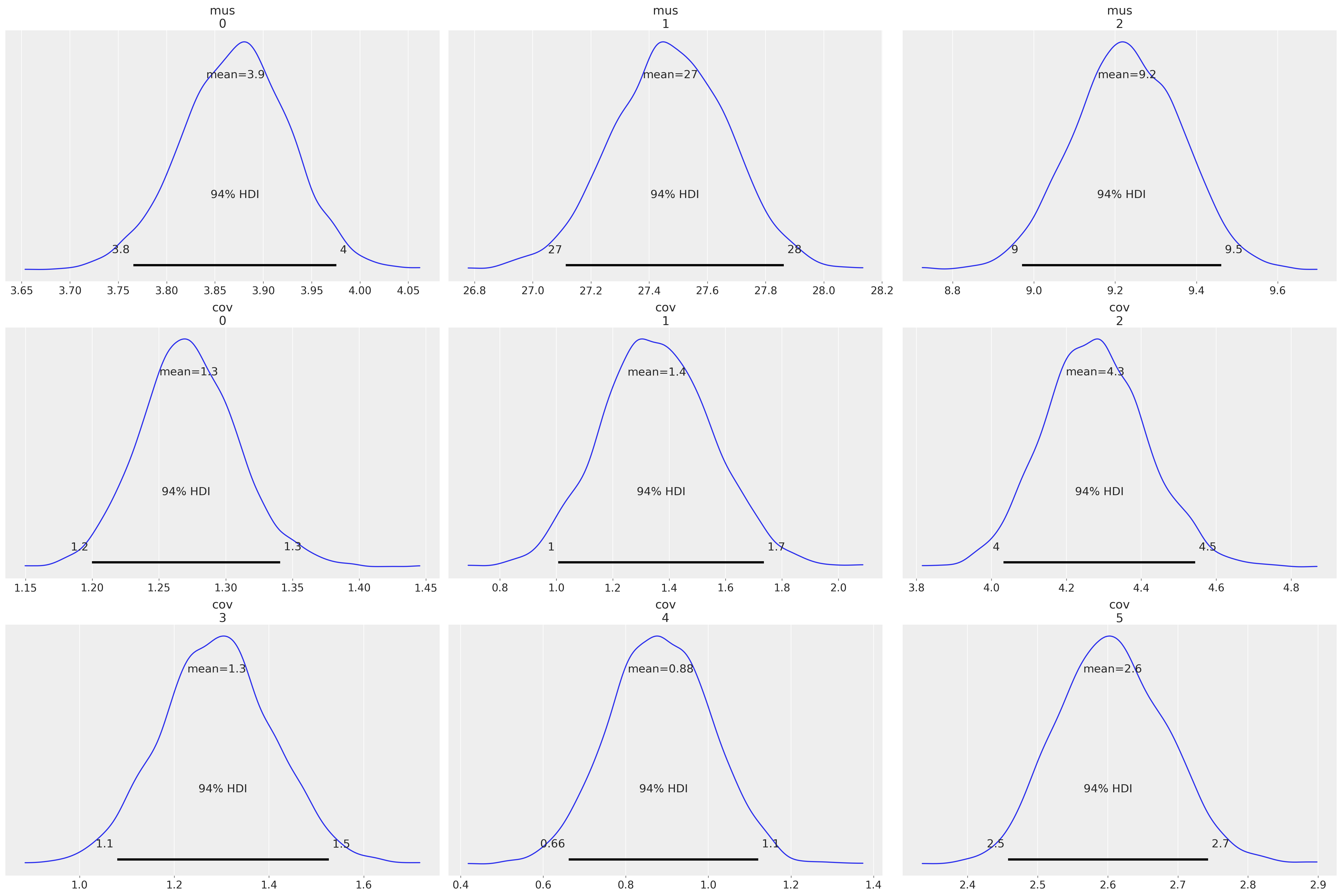
az.summary(idata, var_names=["mus", "cov", "x_unobs"])
| mean | sd | hdi_3% | hdi_97% | mcse_mean | mcse_sd | ess_bulk | ess_tail | r_hat | |
|---|---|---|---|---|---|---|---|---|---|
| mus[0] | 3.871 | 0.056 | 3.766 | 3.976 | 0.001 | 0.001 | 6110.0 | 3277.0 | 1.0 |
| mus[1] | 27.473 | 0.200 | 27.114 | 27.863 | 0.003 | 0.002 | 5742.0 | 3320.0 | 1.0 |
| mus[2] | 9.229 | 0.132 | 8.971 | 9.461 | 0.002 | 0.001 | 6154.0 | 3271.0 | 1.0 |
| cov[0] | 1.272 | 0.037 | 1.200 | 1.341 | 0.000 | 0.000 | 6235.0 | 2754.0 | 1.0 |
| cov[1] | 1.356 | 0.197 | 1.007 | 1.736 | 0.003 | 0.002 | 5373.0 | 3750.0 | 1.0 |
| ... | ... | ... | ... | ... | ... | ... | ... | ... | ... |
| x_unobs[153] | 29.836 | 4.205 | 21.820 | 37.745 | 0.044 | 0.031 | 9232.0 | 2929.0 | 1.0 |
| x_unobs[154] | 2.559 | 1.107 | 0.356 | 4.483 | 0.018 | 0.013 | 3564.0 | 1634.0 | 1.0 |
| x_unobs[155] | 30.071 | 4.029 | 22.614 | 37.652 | 0.039 | 0.028 | 10697.0 | 3078.0 | 1.0 |
| x_unobs[156] | 29.654 | 4.017 | 22.079 | 37.411 | 0.039 | 0.027 | 10626.0 | 2867.0 | 1.0 |
| x_unobs[157] | 27.420 | 4.066 | 19.595 | 34.915 | 0.046 | 0.033 | 7784.0 | 2226.0 | 1.0 |
167 行 × 9 列
imputed_dims = data.shape
imputed = data.values.flatten()
imputed[np.isnan(imputed)] = az.summary(idata, var_names=["x_unobs"])["mean"].values
imputed = imputed.reshape(imputed_dims[0], imputed_dims[1])
imputed = pd.DataFrame(imputed, columns=[col + "_imputed" for col in data.columns])
imputed.head(10)
| worksat_imputed | empower_imputed | lmx_imputed | |
|---|---|---|---|
| 0 | 3.000 | 32.000 | 11.000 |
| 1 | 4.000 | 29.431 | 13.000 |
| 2 | 4.000 | 30.000 | 9.000 |
| 3 | 3.000 | 29.000 | 8.000 |
| 4 | 4.000 | 26.000 | 7.000 |
| 5 | 3.995 | 27.915 | 10.000 |
| 6 | 5.000 | 28.984 | 11.000 |
| 7 | 3.000 | 22.000 | 9.000 |
| 8 | 2.000 | 23.000 | 6.835 |
| 9 | 4.000 | 32.000 | 9.000 |
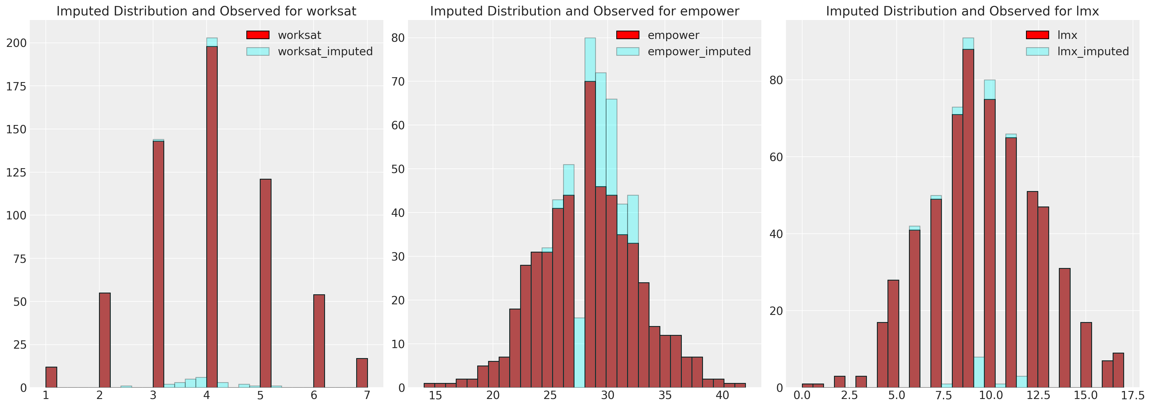
fig, axs = plt.subplots(1, 3, figsize=(20, 7))
axs = axs.flatten()
for col, col_i, ax in zip(data.columns, imputed.columns, axs):
    ax.hist(data[col], color="red", label=col, ec="black", bins=30)
    ax.hist(imputed[col_i], color="cyan", alpha=0.3, label=col_i, ec="black", bins=30)
    ax.legend()
    ax.set_title(f"Imputed Distribution and Observed for {col}")
pd.DataFrame(az.summary(idata, var_names=["cov_corr"])["mean"].values.reshape(3, 3))
/Users/nathanielforde/opt/miniconda3/envs/missing_data_clean/lib/python3.11/site-packages/arviz/stats/diagnostics.py:584: RuntimeWarning: invalid value encountered in scalar divide
  (between_chain_variance / within_chain_variance + num_samples - 1) / (num_samples)
| 0 | 1 | 2 | |
|---|---|---|---|
| 0 | 1.000 | 0.302 | 0.423 |
| 1 | 0.302 | 1.000 | 0.405 |
| 2 | 0.423 | 0.405 | 1.000 |
这些结果与上述FIML方法以及Ender的《应用缺失数据分析》中报告的结果一致。
通过链式方程的贝叶斯插补#
到目前为止,我们已经看到了将数据集中的每个变量视为从同一分布中抽取的集合的多变量插补方法。然而,当我们对某个特定的焦点关系感兴趣时,还有一种更灵活的方法通常很有用。
继续使用员工数据集,我们将在此处研究 lmx、climate、male 和 empower 之间的关系,我们的重点是驱动授权的因素。
请记住,我们的性别变量 male 已完全指定,不需要进行插补。因此,我们有一个可以分解的联合分布:
这可以分解为单独的回归方程,或者更一般地,为每个所需的条件模型分解为组件模型。
我们可以依次对这些方程进行插补,保存插补后的数据集,并将其传递到下一个建模练习中。这增加了一些复杂性,因为一些变量会出现两次。一次作为我们焦点回归中的预测变量,另一次作为它们自己组件模型中的似然项。
PyMC 插补#
正如我们上面所看到的,我们可以使用PyMC通过使用特定的采样分布来填补缺失数据的值。在链式方程的情况下,这变得有点棘手,因为我们可能希望在其中一个方程中将lmx的数据作为回归变量使用,而在另一个方程中将其作为似然函数中的观测数据使用。
我们还关心如何指定用于填补缺失数据的采样分布。我们将在这里展示一个示例,其中我们交替使用均匀和正态采样分布来填补焦点回归中的预测项。
data = df_employee[["lmx", "empower", "climate", "male"]]
lmx_mean = data["lmx"].mean()
lmx_min = data["lmx"].min()
lmx_max = data["lmx"].max()
lmx_sd = data["lmx"].std()

cli_mean = data["climate"].mean()
cli_min = data["climate"].min()
cli_max = data["climate"].max()
cli_sd = data["climate"].std()


priors = {
    "climate": {"normal": [lmx_mean, lmx_sd, lmx_sd], "uniform": [lmx_min, lmx_max]},
    "lmx": {"normal": [cli_mean, cli_sd, cli_sd], "uniform": [cli_min, cli_max]},
}


def make_model(priors, normal_pred_assumption=True):
    coords = {
        "alpha_dim": ["lmx_imputed", "climate_imputed", "empower_imputed"],
        "beta_dim": [
            "lmxB_male",
            "lmxB_climate",
            "climateB_male",
            "empB_male",
            "empB_climate",
            "empB_lmx",
        ],
    }
    with pm.Model(coords=coords) as model:
        # Priors
        beta = pm.Normal("beta", 0, 1, size=6, dims="beta_dim")
        alpha = pm.Normal("alphas", 10, 5, size=3, dims="alpha_dim")
        sigma = pm.HalfNormal("sigmas", 5, size=3, dims="alpha_dim")

        if normal_pred_assumption:
            mu_climate = pm.Normal(
                "mu_climate", priors["climate"]["normal"][0], priors["climate"]["normal"][1]
            )
            sigma_climate = pm.HalfNormal("sigma_climate", priors["climate"]["normal"][2])
            climate_pred = pm.Normal(
                "climate_pred", mu_climate, sigma_climate, observed=data["climate"].values
            )
        else:
            climate_pred = pm.Uniform("climate_pred", 0, 40, observed=data["climate"].values)

        if normal_pred_assumption:
            mu_lmx = pm.Normal("mu_lmx", priors["lmx"]["normal"][0], priors["lmx"]["normal"][1])
            sigma_lmx = pm.HalfNormal("sigma_lmx", priors["lmx"]["normal"][2])
            lmx_pred = pm.Normal("lmx_pred", mu_lmx, sigma_lmx, observed=data["lmx"].values)
        else:
            lmx_pred = pm.Uniform("lmx_pred", 0, 40, observed=data["lmx"].values)

        # Likelihood(s)
        lmx_imputed = pm.Normal(
            "lmx_imputed",
            alpha[0] + beta[0] * data["male"] + beta[1] * climate_pred,
            sigma[0],
            observed=data["lmx"].values,
        )
        climate_imputed = pm.Normal(
            "climate_imputed",
            alpha[1] + beta[2] * data["male"],
            sigma[1],
            observed=data["climate"].values,
        )
        empower_imputed = pm.Normal(
            "emp_imputed",
            alpha[2] + beta[3] * data["male"] + beta[4] * climate_pred + beta[5] * lmx_pred,
            sigma[2],
            observed=data["empower"].values,
        )

        idata = pm.sample_prior_predictive()
        idata.extend(pm.sample(random_seed=120))
        pm.sample_posterior_predictive(idata, extend_inferencedata=True)
        return idata, model


idata_uniform, model_uniform = make_model(priors, normal_pred_assumption=False)
idata_normal, model_normal = make_model(priors, normal_pred_assumption=True)
pm.model_to_graphviz(model_uniform)
/Users/nathanielforde/opt/miniconda3/envs/missing_data_clean/lib/python3.11/site-packages/pymc/model.py:1400: ImputationWarning: Data in climate_pred contains missing values and will be automatically imputed from the sampling distribution.
  warnings.warn(impute_message, ImputationWarning)
/Users/nathanielforde/opt/miniconda3/envs/missing_data_clean/lib/python3.11/site-packages/pymc/model.py:1400: ImputationWarning: Data in lmx_pred contains missing values and will be automatically imputed from the sampling distribution.
  warnings.warn(impute_message, ImputationWarning)
/Users/nathanielforde/opt/miniconda3/envs/missing_data_clean/lib/python3.11/site-packages/pymc/model.py:1400: ImputationWarning: Data in lmx_imputed contains missing values and will be automatically imputed from the sampling distribution.
  warnings.warn(impute_message, ImputationWarning)
/Users/nathanielforde/opt/miniconda3/envs/missing_data_clean/lib/python3.11/site-packages/pymc/model.py:1400: ImputationWarning: Data in climate_imputed contains missing values and will be automatically imputed from the sampling distribution.
  warnings.warn(impute_message, ImputationWarning)
/Users/nathanielforde/opt/miniconda3/envs/missing_data_clean/lib/python3.11/site-packages/pymc/model.py:1400: ImputationWarning: Data in emp_imputed contains missing values and will be automatically imputed from the sampling distribution.
  warnings.warn(impute_message, ImputationWarning)
Sampling: [alphas, beta, climate_imputed_missing, climate_imputed_observed, climate_pred_missing, climate_pred_observed, emp_imputed_missing, emp_imputed_observed, lmx_imputed_missing, lmx_imputed_observed, lmx_pred_missing, lmx_pred_observed, sigmas]
Auto-assigning NUTS sampler...
Initializing NUTS using jitter+adapt_diag...
Multiprocess sampling (4 chains in 4 jobs)
NUTS: [beta, alphas, sigmas, climate_pred_missing, lmx_pred_missing, lmx_imputed_missing, climate_imputed_missing, emp_imputed_missing]
Sampling 4 chains for 1_000 tune and 1_000 draw iterations (4_000 + 4_000 draws total) took 96 seconds.
Sampling: [climate_imputed_observed, climate_pred_observed, emp_imputed_missing, emp_imputed_observed, lmx_imputed_missing, lmx_imputed_observed, lmx_pred_observed]
/Users/nathanielforde/opt/miniconda3/envs/missing_data_clean/lib/python3.11/site-packages/pymc/model.py:1400: ImputationWarning: Data in climate_pred contains missing values and will be automatically imputed from the sampling distribution.
  warnings.warn(impute_message, ImputationWarning)
/Users/nathanielforde/opt/miniconda3/envs/missing_data_clean/lib/python3.11/site-packages/pymc/model.py:1400: ImputationWarning: Data in lmx_pred contains missing values and will be automatically imputed from the sampling distribution.
  warnings.warn(impute_message, ImputationWarning)
/Users/nathanielforde/opt/miniconda3/envs/missing_data_clean/lib/python3.11/site-packages/pymc/model.py:1400: ImputationWarning: Data in lmx_imputed contains missing values and will be automatically imputed from the sampling distribution.
  warnings.warn(impute_message, ImputationWarning)
/Users/nathanielforde/opt/miniconda3/envs/missing_data_clean/lib/python3.11/site-packages/pymc/model.py:1400: ImputationWarning: Data in climate_imputed contains missing values and will be automatically imputed from the sampling distribution.
  warnings.warn(impute_message, ImputationWarning)
/Users/nathanielforde/opt/miniconda3/envs/missing_data_clean/lib/python3.11/site-packages/pymc/model.py:1400: ImputationWarning: Data in emp_imputed contains missing values and will be automatically imputed from the sampling distribution.
  warnings.warn(impute_message, ImputationWarning)
Sampling: [alphas, beta, climate_imputed_missing, climate_imputed_observed, climate_pred_missing, climate_pred_observed, emp_imputed_missing, emp_imputed_observed, lmx_imputed_missing, lmx_imputed_observed, lmx_pred_missing, lmx_pred_observed, mu_climate, mu_lmx, sigma_climate, sigma_lmx, sigmas]
Auto-assigning NUTS sampler...
Initializing NUTS using jitter+adapt_diag...
Multiprocess sampling (4 chains in 4 jobs)
NUTS: [beta, alphas, sigmas, mu_climate, sigma_climate, climate_pred_missing, mu_lmx, sigma_lmx, lmx_pred_missing, lmx_imputed_missing, climate_imputed_missing, emp_imputed_missing]
Sampling 4 chains for 1_000 tune and 1_000 draw iterations (4_000 + 4_000 draws total) took 106 seconds.
Sampling: [climate_imputed_observed, climate_pred_observed, emp_imputed_missing, emp_imputed_observed, lmx_imputed_missing, lmx_imputed_observed, lmx_pred_observed]

idata_normal
-
<xarray.Dataset> Dimensions: (chain: 4, draw: 1000, beta_dim: 6, alpha_dim: 3, climate_pred_missing_dim_0: 60, lmx_pred_missing_dim_0: 26, lmx_imputed_missing_dim_0: 26, climate_imputed_missing_dim_0: 60, emp_imputed_missing_dim_0: 102, climate_pred_dim_0: 630, lmx_pred_dim_0: 630, lmx_imputed_dim_0: 630, climate_imputed_dim_0: 630, emp_imputed_dim_0: 630) Coordinates: (12/14) * chain (chain) int64 0 1 2 3 * draw (draw) int64 0 1 2 3 4 ... 996 997 998 999 * beta_dim (beta_dim) <U13 'lmxB_male' ... 'empB_lmx' * alpha_dim (alpha_dim) <U15 'lmx_imputed' ... 'empowe... * climate_pred_missing_dim_0 (climate_pred_missing_dim_0) int64 0 1 ... 59 * lmx_pred_missing_dim_0 (lmx_pred_missing_dim_0) int64 0 1 ... 24 25 ... ... * emp_imputed_missing_dim_0 (emp_imputed_missing_dim_0) int64 0 1 ... 101 * climate_pred_dim_0 (climate_pred_dim_0) int64 0 1 2 ... 628 629 * lmx_pred_dim_0 (lmx_pred_dim_0) int64 0 1 2 ... 627 628 629 * lmx_imputed_dim_0 (lmx_imputed_dim_0) int64 0 1 2 ... 628 629 * climate_imputed_dim_0 (climate_imputed_dim_0) int64 0 1 ... 628 629 * emp_imputed_dim_0 (emp_imputed_dim_0) int64 0 1 2 ... 628 629 Data variables: (12/17) beta (chain, draw, beta_dim) float64 0.5683 ...... alphas (chain, draw, alpha_dim) float64 9.008 ...... mu_climate (chain, draw) float64 19.98 20.11 ... 20.12 climate_pred_missing (chain, draw, climate_pred_missing_dim_0) float64 ... mu_lmx (chain, draw) float64 9.514 9.723 ... 9.586 lmx_pred_missing (chain, draw, lmx_pred_missing_dim_0) float64 ... ... ... sigma_lmx (chain, draw) float64 3.027 3.152 ... 3.004 climate_pred (chain, draw, climate_pred_dim_0) float64 ... lmx_pred (chain, draw, lmx_pred_dim_0) float64 11.0... lmx_imputed (chain, draw, lmx_imputed_dim_0) float64 1... climate_imputed (chain, draw, climate_imputed_dim_0) float64 ... emp_imputed (chain, draw, emp_imputed_dim_0) float64 3... Attributes: created_at: 2023-02-02T07:57:06.498924 arviz_version: 0.14.0 inference_library: pymc inference_library_version: 5.0.1 sampling_time: 106.22190403938293 tuning_steps: 1000 -
<xarray.Dataset> Dimensions: (chain: 4, draw: 1000, climate_pred_observed_dim_2: 570, lmx_pred_observed_dim_2: 604, lmx_imputed_observed_dim_2: 604, climate_imputed_observed_dim_2: 570, emp_imputed_observed_dim_2: 528, climate_pred_dim_2: 630, lmx_pred_dim_2: 630, lmx_imputed_dim_2: 630, climate_imputed_dim_2: 630, emp_imputed_dim_2: 630) Coordinates: * chain (chain) int64 0 1 2 3 * draw (draw) int64 0 1 2 3 4 ... 996 997 998 999 * climate_pred_observed_dim_2 (climate_pred_observed_dim_2) int64 0 ...... * lmx_pred_observed_dim_2 (lmx_pred_observed_dim_2) int64 0 1 ... 603 * lmx_imputed_observed_dim_2 (lmx_imputed_observed_dim_2) int64 0 ... 603 * climate_imputed_observed_dim_2 (climate_imputed_observed_dim_2) int64 0 ... * emp_imputed_observed_dim_2 (emp_imputed_observed_dim_2) int64 0 ... 527 * climate_pred_dim_2 (climate_pred_dim_2) int64 0 1 2 ... 628 629 * lmx_pred_dim_2 (lmx_pred_dim_2) int64 0 1 2 ... 627 628 629 * lmx_imputed_dim_2 (lmx_imputed_dim_2) int64 0 1 2 ... 628 629 * climate_imputed_dim_2 (climate_imputed_dim_2) int64 0 1 ... 629 * emp_imputed_dim_2 (emp_imputed_dim_2) int64 0 1 2 ... 628 629 Data variables: climate_pred_observed (chain, draw, climate_pred_observed_dim_2) float64 ... lmx_pred_observed (chain, draw, lmx_pred_observed_dim_2) float64 ... lmx_imputed_observed (chain, draw, lmx_imputed_observed_dim_2) float64 ... climate_imputed_observed (chain, draw, climate_imputed_observed_dim_2) float64 ... emp_imputed_observed (chain, draw, emp_imputed_observed_dim_2) float64 ... climate_pred (chain, draw, climate_pred_dim_2) float64 ... lmx_pred (chain, draw, lmx_pred_dim_2) float64 8.6... lmx_imputed (chain, draw, lmx_imputed_dim_2) float64 ... climate_imputed (chain, draw, climate_imputed_dim_2) float64 ... emp_imputed (chain, draw, emp_imputed_dim_2) float64 ... Attributes: created_at: 2023-02-02T07:57:11.095286 arviz_version: 0.14.0 inference_library: pymc inference_library_version: 5.0.1 -
<xarray.Dataset> Dimensions: (chain: 4, draw: 1000) Coordinates: * chain (chain) int64 0 1 2 3 * draw (draw) int64 0 1 2 3 4 5 ... 994 995 996 997 998 999 Data variables: (12/17) n_steps (chain, draw) float64 31.0 31.0 31.0 ... 31.0 31.0 max_energy_error (chain, draw) float64 -0.3783 -0.1605 ... 0.6239 diverging (chain, draw) bool False False False ... False False reached_max_treedepth (chain, draw) bool False False False ... False False acceptance_rate (chain, draw) float64 0.9975 0.9587 ... 0.6311 0.7695 process_time_diff (chain, draw) float64 0.02338 0.02421 ... 0.01917 ... ... perf_counter_start (chain, draw) float64 4.427e+05 ... 4.427e+05 energy (chain, draw) float64 8.642e+03 ... 8.615e+03 lp (chain, draw) float64 -8.501e+03 ... -8.471e+03 energy_error (chain, draw) float64 -0.1605 0.1162 ... -0.08054 largest_eigval (chain, draw) float64 nan nan nan nan ... nan nan nan tree_depth (chain, draw) int64 5 5 5 5 5 5 5 5 ... 5 5 5 5 5 5 5 Attributes: created_at: 2023-02-02T07:57:06.518637 arviz_version: 0.14.0 inference_library: pymc inference_library_version: 5.0.1 sampling_time: 106.22190403938293 tuning_steps: 1000 -
<xarray.Dataset> Dimensions: (chain: 1, draw: 500, alpha_dim: 3, beta_dim: 6, climate_pred_missing_dim_0: 60, climate_imputed_missing_dim_0: 60, emp_imputed_dim_0: 630, climate_imputed_dim_0: 630, lmx_pred_dim_0: 630, lmx_imputed_missing_dim_0: 26, emp_imputed_missing_dim_0: 102, lmx_pred_missing_dim_0: 26, lmx_imputed_dim_0: 630, climate_pred_dim_0: 630) Coordinates: (12/14) * chain (chain) int64 0 * draw (draw) int64 0 1 2 3 4 ... 496 497 498 499 * alpha_dim (alpha_dim) <U15 'lmx_imputed' ... 'empowe... * beta_dim (beta_dim) <U13 'lmxB_male' ... 'empB_lmx' * climate_pred_missing_dim_0 (climate_pred_missing_dim_0) int64 0 1 ... 59 * climate_imputed_missing_dim_0 (climate_imputed_missing_dim_0) int64 0 ..... ... ... * lmx_pred_dim_0 (lmx_pred_dim_0) int64 0 1 2 ... 627 628 629 * lmx_imputed_missing_dim_0 (lmx_imputed_missing_dim_0) int64 0 1 ... 25 * emp_imputed_missing_dim_0 (emp_imputed_missing_dim_0) int64 0 1 ... 101 * lmx_pred_missing_dim_0 (lmx_pred_missing_dim_0) int64 0 1 ... 24 25 * lmx_imputed_dim_0 (lmx_imputed_dim_0) int64 0 1 2 ... 628 629 * climate_pred_dim_0 (climate_pred_dim_0) int64 0 1 2 ... 628 629 Data variables: (12/17) alphas (chain, draw, alpha_dim) float64 11.45 ...... sigma_climate (chain, draw) float64 1.15 0.4145 ... 0.8882 beta (chain, draw, beta_dim) float64 1.199 ... ... climate_pred_missing (chain, draw, climate_pred_missing_dim_0) float64 ... climate_imputed_missing (chain, draw, climate_imputed_missing_dim_0) float64 ... emp_imputed (chain, draw, emp_imputed_dim_0) float64 8... ... ... sigmas (chain, draw, alpha_dim) float64 6.3 ... 1... lmx_pred_missing (chain, draw, lmx_pred_missing_dim_0) float64 ... sigma_lmx (chain, draw) float64 1.127 5.054 ... 6.724 lmx_imputed (chain, draw, lmx_imputed_dim_0) float64 2... mu_climate (chain, draw) float64 4.559 9.647 ... 9.476 climate_pred (chain, draw, climate_pred_dim_0) float64 ... Attributes: created_at: 2023-02-02T07:54:57.199499 arviz_version: 0.14.0 inference_library: pymc inference_library_version: 5.0.1 -
<xarray.Dataset> Dimensions: (chain: 1, draw: 500, lmx_pred_observed_dim_0: 604, emp_imputed_observed_dim_0: 528, lmx_imputed_observed_dim_0: 604, climate_imputed_observed_dim_0: 570, climate_pred_observed_dim_0: 570) Coordinates: * chain (chain) int64 0 * draw (draw) int64 0 1 2 3 4 ... 496 497 498 499 * lmx_pred_observed_dim_0 (lmx_pred_observed_dim_0) int64 0 1 ... 603 * emp_imputed_observed_dim_0 (emp_imputed_observed_dim_0) int64 0 ... 527 * lmx_imputed_observed_dim_0 (lmx_imputed_observed_dim_0) int64 0 ... 603 * climate_imputed_observed_dim_0 (climate_imputed_observed_dim_0) int64 0 ... * climate_pred_observed_dim_0 (climate_pred_observed_dim_0) int64 0 ...... Data variables: lmx_pred_observed (chain, draw, lmx_pred_observed_dim_0) float64 ... emp_imputed_observed (chain, draw, emp_imputed_observed_dim_0) float64 ... lmx_imputed_observed (chain, draw, lmx_imputed_observed_dim_0) float64 ... climate_imputed_observed (chain, draw, climate_imputed_observed_dim_0) float64 ... climate_pred_observed (chain, draw, climate_pred_observed_dim_0) float64 ... Attributes: created_at: 2023-02-02T07:54:57.206651 arviz_version: 0.14.0 inference_library: pymc inference_library_version: 5.0.1 -
<xarray.Dataset>
Dimensions:                         (climate_pred_observed_dim_0: 570,
                                     lmx_pred_observed_dim_0: 604,
                                     lmx_imputed_observed_dim_0: 604,
                                     climate_imputed_observed_dim_0: 570,
                                     emp_imputed_observed_dim_0: 528)
Coordinates:
  * climate_pred_observed_dim_0     (climate_pred_observed_dim_0) int64 0 ......
  * lmx_pred_observed_dim_0         (lmx_pred_observed_dim_0) int64 0 1 ... 603
  * lmx_imputed_observed_dim_0      (lmx_imputed_observed_dim_0) int64 0 ... 603
  * climate_imputed_observed_dim_0  (climate_imputed_observed_dim_0) int64 0 ...
  * emp_imputed_observed_dim_0      (emp_imputed_observed_dim_0) int64 0 ... 527
Data variables:
    climate_pred_observed           (climate_pred_observed_dim_0) float64 18....
    lmx_pred_observed               (lmx_pred_observed_dim_0) float64 11.0 .....
    lmx_imputed_observed            (lmx_imputed_observed_dim_0) float64 11.0...
    climate_imputed_observed        (climate_imputed_observed_dim_0) float64 ...
    emp_imputed_observed            (emp_imputed_observed_dim_0) float64 32.0...
Attributes:
    created_at:                 2023-02-02T07:54:57.209280
    arviz_version:              0.14.0
    inference_library:          pymc
    inference_library_version:  5.0.1
模型拟合#
接下来我们将检查回归模型的参数拟合情况,并观察它们如何依赖于插补方案中的先验规范。
az.summary(idata_normal, var_names=["alphas", "beta", "sigmas"], stat_focus="median")
| median | mad | eti_3% | eti_97% | mcse_median | ess_median | ess_tail | r_hat | |
|---|---|---|---|---|---|---|---|---|
| alphas[lmx_imputed] | 9.057 | 0.446 | 7.854 | 10.263 | 0.011 | 3920.446 | 3077.0 | 1.00 |
| alphas[climate_imputed] | 19.776 | 0.158 | 19.345 | 20.213 | 0.005 | 4203.071 | 3452.0 | 1.00 |
| alphas[empower_imputed] | 17.928 | 0.689 | 16.016 | 19.851 | 0.022 | 3143.699 | 3063.0 | 1.00 |
| beta[lmxB_male] | 0.437 | 0.157 | -0.005 | 0.894 | 0.003 | 7104.804 | 3102.0 | 1.00 |
| beta[lmxB_climate] | 0.018 | 0.022 | -0.042 | 0.076 | 0.001 | 3670.069 | 2911.0 | 1.00 |
| beta[climateB_male] | 0.696 | 0.214 | 0.092 | 1.286 | 0.006 | 4471.550 | 3328.0 | 1.00 |
| beta[empB_male] | 1.656 | 0.214 | 1.043 | 2.254 | 0.005 | 5282.112 | 3361.0 | 1.00 |
| beta[empB_climate] | 0.203 | 0.030 | 0.121 | 0.286 | 0.001 | 3395.600 | 3068.0 | 1.00 |
| beta[empB_lmx] | 0.598 | 0.039 | 0.489 | 0.710 | 0.001 | 4541.732 | 2991.0 | 1.00 |
| sigmas[lmx_imputed] | 3.023 | 0.059 | 2.865 | 3.199 | 0.001 | 5408.426 | 3360.0 | 1.00 |
| sigmas[climate_imputed] | 4.021 | 0.077 | 3.812 | 4.251 | 0.002 | 5084.700 | 3347.0 | 1.01 |
| sigmas[empower_imputed] | 3.815 | 0.079 | 3.598 | 4.052 | 0.002 | 4530.686 | 3042.0 | 1.00 |
az.summary(idata_uniform, var_names=["alphas", "beta", "sigmas"], stat_focus="median")
| median | mad | eti_3% | eti_97% | mcse_median | ess_median | ess_tail | r_hat | |
|---|---|---|---|---|---|---|---|---|
| alphas[lmx_imputed] | 9.159 | 0.402 | 8.082 | 10.230 | 0.015 | 3450.523 | 3292.0 | 1.0 |
| alphas[climate_imputed] | 19.781 | 0.159 | 19.339 | 20.219 | 0.004 | 4512.068 | 3360.0 | 1.0 |
| alphas[empower_imputed] | 18.855 | 0.645 | 17.070 | 20.708 | 0.026 | 2292.646 | 2706.0 | 1.0 |
| beta[lmxB_male] | 0.433 | 0.166 | 0.013 | 0.867 | 0.003 | 6325.253 | 3040.0 | 1.0 |
| beta[lmxB_climate] | 0.013 | 0.019 | -0.039 | 0.065 | 0.001 | 3197.124 | 3042.0 | 1.0 |
| beta[climateB_male] | 0.689 | 0.224 | 0.067 | 1.284 | 0.006 | 4576.652 | 3231.0 | 1.0 |
| beta[empB_male] | 1.625 | 0.215 | 1.025 | 2.230 | 0.005 | 6056.623 | 3056.0 | 1.0 |
| beta[empB_climate] | 0.206 | 0.025 | 0.130 | 0.275 | 0.001 | 3166.040 | 2923.0 | 1.0 |
| beta[empB_lmx] | 0.488 | 0.044 | 0.363 | 0.608 | 0.001 | 2428.278 | 2756.0 | 1.0 |
| sigmas[lmx_imputed] | 3.020 | 0.058 | 2.874 | 3.186 | 0.001 | 7159.549 | 3040.0 | 1.0 |
| sigmas[climate_imputed] | 4.018 | 0.081 | 3.808 | 4.252 | 0.002 | 6092.150 | 2921.0 | 1.0 |
| sigmas[empower_imputed] | 3.783 | 0.082 | 3.572 | 4.029 | 0.002 | 4046.865 | 2845.0 | 1.0 |
我们可以看到,采样分布的选择如何在我们两个模型中对beta系数的参数估计产生了不同的影响。这两个插补在参数层面上大致一致,但它们在含义上存在显著差异。
az.plot_forest(
    [idata_normal, idata_uniform],
    var_names=["beta"],
    kind="ridgeplot",
    model_names=["Gaussian Sampling Distribution", "Uniform Sampling Distribution"],
    figsize=(10, 8),
)
array([<AxesSubplot: >], dtype=object)
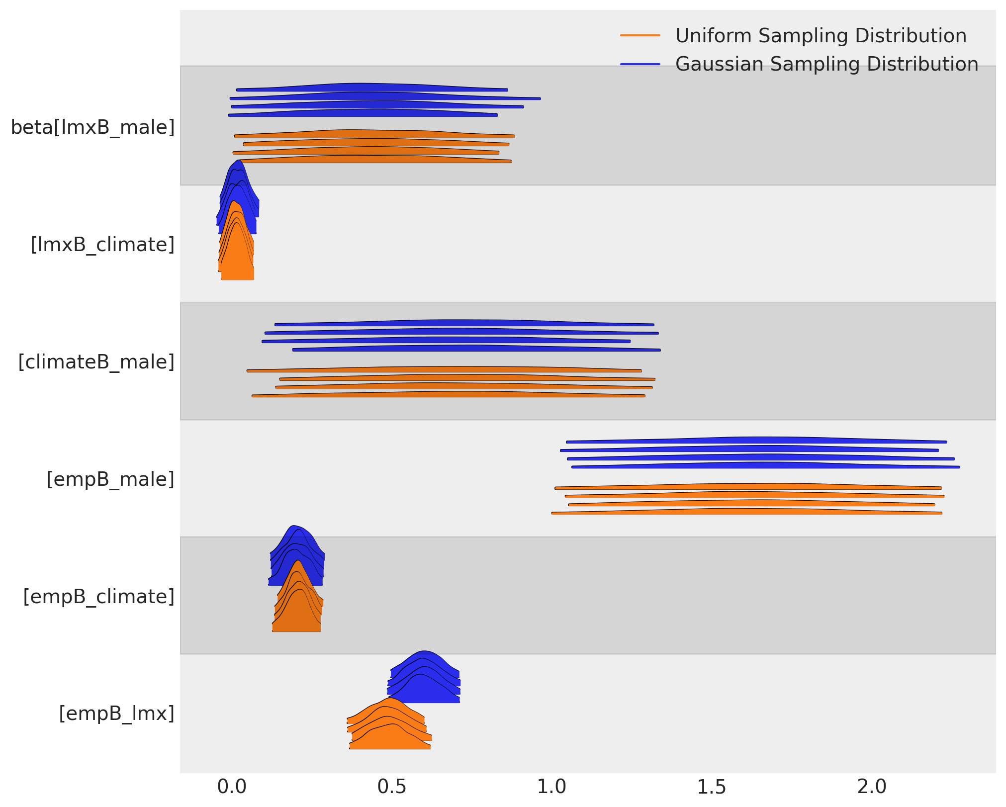
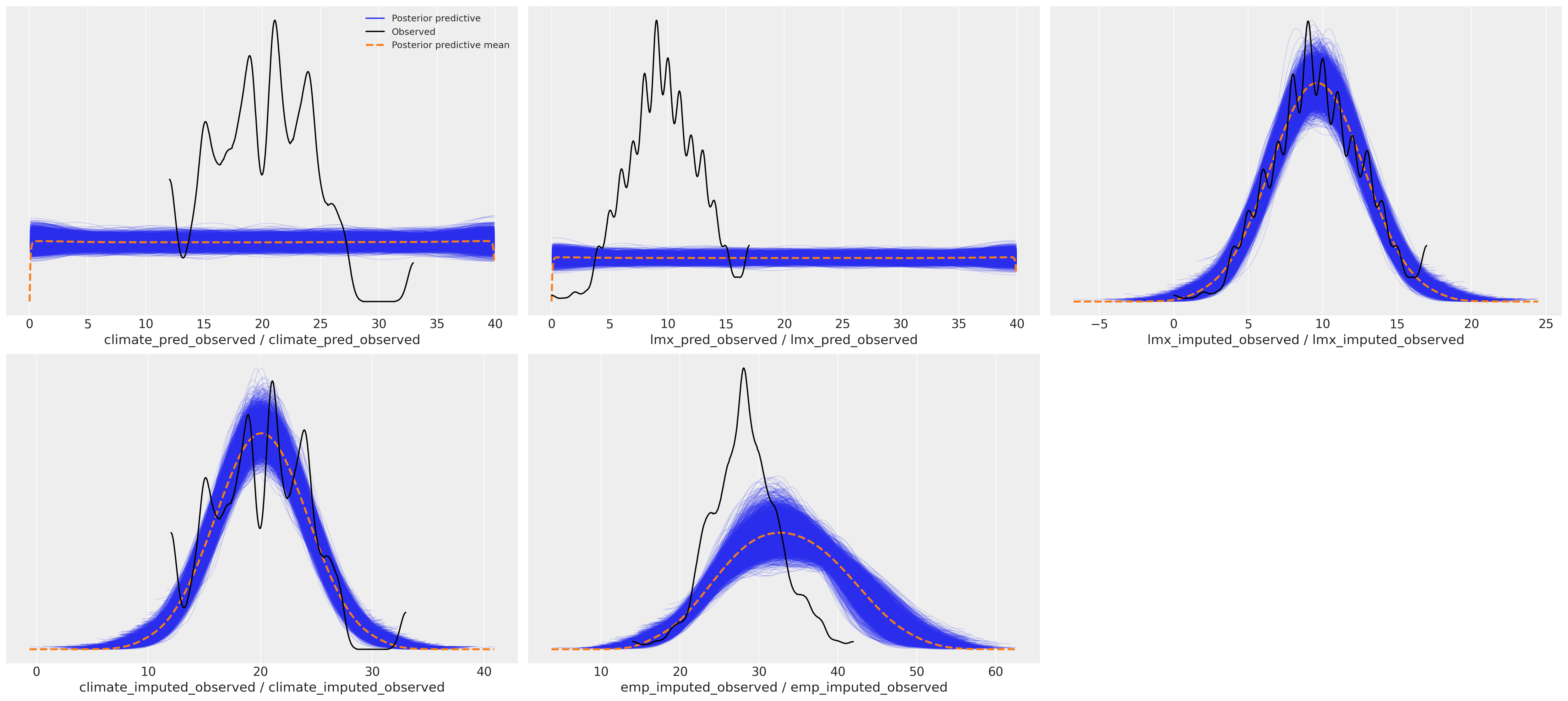
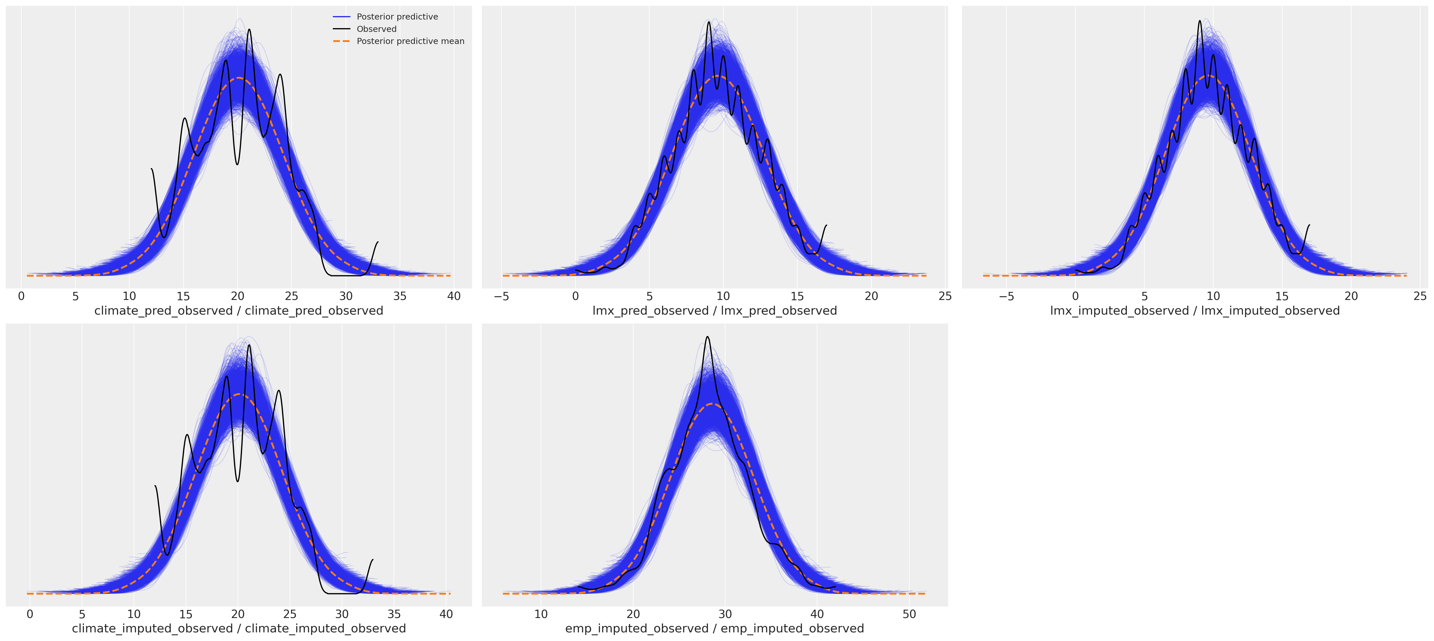
这种差异对后验预测分布产生了下游影响。我们可以在这里看到预测项的采样分布如何影响我们焦点回归方程的后验预测拟合。
后验预测分布#
az.plot_ppc(idata_uniform)
array([[<AxesSubplot: xlabel='climate_pred_observed / climate_pred_observed'>,
        <AxesSubplot: xlabel='lmx_pred_observed / lmx_pred_observed'>,
        <AxesSubplot: xlabel='lmx_imputed_observed / lmx_imputed_observed'>],
       [<AxesSubplot: xlabel='climate_imputed_observed / climate_imputed_observed'>,
        <AxesSubplot: xlabel='emp_imputed_observed / emp_imputed_observed'>,
        <AxesSubplot: >]], dtype=object)
az.plot_ppc(idata_normal)
array([[<AxesSubplot: xlabel='climate_pred_observed / climate_pred_observed'>,
        <AxesSubplot: xlabel='lmx_pred_observed / lmx_pred_observed'>,
        <AxesSubplot: xlabel='lmx_imputed_observed / lmx_imputed_observed'>],
       [<AxesSubplot: xlabel='climate_imputed_observed / climate_imputed_observed'>,
        <AxesSubplot: xlabel='emp_imputed_observed / emp_imputed_observed'>,
        <AxesSubplot: >]], dtype=object)
处理后验预测分布#
在上文中,我们在一个PyMC模型上下文中估计了许多似然项。这些似然项约束了超参数,这些超参数决定了在我们关注的回归方程中用作预测变量的变量中缺失项的填补值。但我们也可以执行更手动化的顺序填补,其中我们分别对每个从属回归方程进行建模,并依次提取每个变量的填补值,然后对关注回归方程的填补值进行简单回归。
我们在这里展示如何提取每个回归方程的插补值并增强观测数据。
def get_imputed(idata, data):
    imputed_data = data.copy()
    imputed_climate = az.extract(idata, group="posterior_predictive", num_samples=1000)[
        "climate_imputed"
    ].mean(axis=1)
    mask = imputed_data["climate"].isnull()
    imputed_data.loc[mask, "climate"] = imputed_climate.values[imputed_data[mask].index]

    imputed_lmx = az.extract(idata, group="posterior_predictive", num_samples=1000)[
        "lmx_imputed"
    ].mean(axis=1)
    mask = imputed_data["lmx"].isnull()
    imputed_data.loc[mask, "lmx"] = imputed_lmx.values[imputed_data[mask].index]

    imputed_emp = az.extract(idata, group="posterior_predictive", num_samples=1000)[
        "emp_imputed"
    ].mean(axis=1)
    mask = imputed_data["empower"].isnull()
    imputed_data.loc[mask, "empower"] = imputed_emp.values[imputed_data[mask].index]
    assert imputed_data.isnull().sum().to_list() == [0, 0, 0, 0]
    imputed_data.columns = ["imputed_" + col for col in imputed_data.columns]
    return imputed_data


imputed_data_uniform = get_imputed(idata_uniform, data)
imputed_data_normal = get_imputed(idata_normal, data)
imputed_data_normal.head(5)
| imputed_lmx | imputed_empower | imputed_climate | imputed_male | |
|---|---|---|---|---|
| 0 | 11.0 | 32.000000 | 18.0 | 1 |
| 1 | 13.0 | 29.490539 | 18.0 | 1 |
| 2 | 9.0 | 30.000000 | 18.0 | 1 |
| 3 | 8.0 | 29.000000 | 18.0 | 1 |
| 4 | 7.0 | 26.000000 | 18.0 | 0 |
我们在这里使用均值来填补每个缺失单元格的期望值,但你可以使用后验预测分布中的许多合理值来进行某种敏感性分析
绘制插补数据集#
现在我们将绘制插补值与其观测值的关系图,以展示不同的采样分布如何影响插补的模式。
joined_uniform = pd.concat([imputed_data_uniform, data], axis=1)
joined_normal = pd.concat([imputed_data_normal, data], axis=1)
for col in ["lmx", "empower", "climate"]:
    joined_uniform[col + "_missing"] = np.where(joined_uniform[col].isnull(), 1, 0)
    joined_normal[col + "_missing"] = np.where(joined_normal[col].isnull(), 1, 0)


def rand_jitter(arr):
    stdev = 0.01 * (max(arr) - min(arr))
    return arr + np.random.randn(len(arr)) * stdev


fig, axs = plt.subplots(1, 3, figsize=(20, 8))
axs = axs.flatten()
ax = axs[0]
ax1 = axs[1]
ax2 = axs[2]

## Derived from MV norm fit.
z = multivariate_normal(
    [lmx_mean, joined_uniform["imputed_empower"].mean()], [[8.9, 5.4], [5.4, 19]]
).pdf(joined_uniform[["imputed_lmx", "imputed_empower"]])

ax.scatter(
    rand_jitter(joined_uniform["imputed_lmx"]),
    rand_jitter(joined_uniform["imputed_empower"]),
    c=joined_uniform["empower_missing"],
    cmap=cm.winter,
    ec="black",
    s=50,
)
ax.set_title("Relationship between LMX and Empowerment \n after Uniform Imputation", fontsize=20)
ax.tricontour(joined_uniform["imputed_lmx"], joined_uniform["imputed_empower"], z)
ax.set_xlabel("Leader-Member-Exchange")
ax.set_ylabel("Empowerment")


custom_lines = [
    Line2D([0], [0], color=cm.winter(0.0), lw=4),
    Line2D([0], [0], color=cm.winter(0.9), lw=4),
]
ax.legend(custom_lines, ["Observed", "Missing - Imputed Empowerment Values"])

z = multivariate_normal(
    [lmx_mean, joined_normal["imputed_empower"].mean()], [[8.9, 5.4], [5.4, 19]]
).pdf(joined_normal[["imputed_lmx", "imputed_empower"]])

ax2.scatter(
    rand_jitter(joined_normal["imputed_lmx"]),
    rand_jitter(joined_normal["imputed_empower"]),
    c=joined_normal["empower_missing"],
    cmap=cm.autumn,
    ec="black",
    s=50,
)
ax2.set_title("Relationship between LMX and Empowerment \n after Gaussian Imputation", fontsize=20)
ax2.tricontour(joined_normal["imputed_lmx"], joined_normal["imputed_empower"], z)
ax2.set_xlabel("Leader-Member-Exchange")
ax2.set_ylabel("Empowerment")
custom_lines = [
    Line2D([0], [0], color=cm.autumn(0.0), lw=4),
    Line2D([0], [0], color=cm.autumn(0.9), lw=4),
]
ax2.legend(custom_lines, ["Observed", "Missing - Imputed Empowerment Values"])

ax1.hist(
    joined_normal["imputed_empower"],
    label="Gaussian Imputed Empowerment",
    bins=30,
    color="slateblue",
    ec="black",
)
ax1.hist(
    joined_uniform["imputed_empower"],
    label="Uniform Imputed Empowerment",
    bins=30,
    color="cyan",
    ec="black",
)
ax1.hist(
    joined_normal["empower"], label="Observed Empowerment", bins=30, color="magenta", ec="black"
)
ax1.legend()
ax1.set_title("Imputed & Observed Empowerment", fontsize=20);
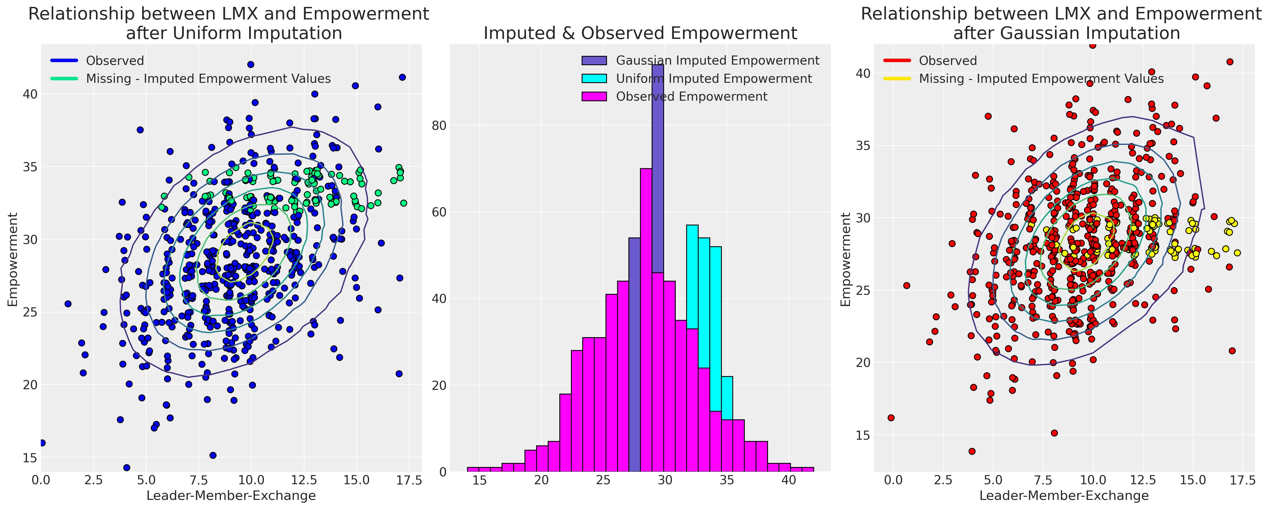
最终,我们对采样分布的选择导致了不同可能性的插补。选择哪种模型将由支配我们数据中缺失原因的假设所驱动。
层次结构和数据插补#
我们的员工数据集比我们迄今为止所研究的具有更细致的结构。特别是,有大约100个团队组成了我们的员工群体,我们可能会想知道满意度或不完全调查分数在多大程度上是由于当地团队环境造成的?这可能是我们缺失数据模式的一个因素吗?我们将通过团队检查报告的授权分数,并根据每个团队报告的lmx分数绘制回归线。
heatmap = df_employee.pivot("employee", "team", "empower").dropna(how="all")
heatmap = pd.concat(
    [heatmap[~heatmap[col].isnull()][col].reset_index(drop=True) for col in heatmap.columns], axis=1
)
with pd.option_context("format.precision", 2):
    display(heatmap.style.background_gradient(cmap="Blues"));
/var/folders/99/gp2xl6x513s0tvl3cx79zf7m0000gn/T/ipykernel_96943/1805800404.py:1: FutureWarning: In a future version of pandas all arguments of DataFrame.pivot will be keyword-only.
  heatmap = df_employee.pivot("employee", "team", "empower").dropna(how="all")
| 1 | 2 | 3 | 4 | 5 | 6 | 7 | 8 | 9 | 10 | 11 | 12 | 13 | 14 | 15 | 16 | 17 | 18 | 19 | 20 | 21 | 22 | 23 | 24 | 25 | 26 | 27 | 28 | 29 | 30 | 31 | 32 | 33 | 34 | 35 | 36 | 37 | 38 | 39 | 40 | 41 | 42 | 43 | 44 | 45 | 46 | 47 | 48 | 49 | 50 | 51 | 52 | 53 | 54 | 55 | 56 | 57 | 58 | 59 | 60 | 61 | 62 | 63 | 64 | 65 | 66 | 67 | 68 | 69 | 70 | 71 | 72 | 73 | 74 | 75 | 76 | 77 | 78 | 79 | 80 | 81 | 82 | 83 | 84 | 85 | 86 | 87 | 88 | 89 | 90 | 91 | 92 | 93 | 94 | 95 | 96 | 97 | 98 | 99 | 100 | 101 | 102 | 103 | 104 | 105 | |
|---|---|---|---|---|---|---|---|---|---|---|---|---|---|---|---|---|---|---|---|---|---|---|---|---|---|---|---|---|---|---|---|---|---|---|---|---|---|---|---|---|---|---|---|---|---|---|---|---|---|---|---|---|---|---|---|---|---|---|---|---|---|---|---|---|---|---|---|---|---|---|---|---|---|---|---|---|---|---|---|---|---|---|---|---|---|---|---|---|---|---|---|---|---|---|---|---|---|---|---|---|---|---|---|---|---|
| 0 | 32.00 | 22.00 | 16.00 | 26.00 | 33.00 | 21.00 | 29.00 | 26.00 | 27.00 | 33.00 | 28.00 | 36.00 | 24.00 | 24.00 | 34.00 | 28.00 | 29.00 | 22.00 | 28.00 | 23.00 | 25.00 | 39.00 | 28.00 | 28.00 | 26.00 | 29.00 | 34.00 | 25.00 | 30.00 | 26.00 | 28.00 | 23.00 | 32.00 | 27.00 | 38.00 | 22.00 | 36.00 | 30.00 | 30.00 | 30.00 | 30.00 | 28.00 | 27.00 | 28.00 | 25.00 | 21.00 | 37.00 | 24.00 | 31.00 | 27.00 | 28.00 | 32.00 | 27.00 | 30.00 | 28.00 | 26.00 | 29.00 | 20.00 | 30.00 | 27.00 | 32.00 | 22.00 | 32.00 | 31.00 | 26.00 | 29.00 | 24.00 | 23.00 | 33.00 | 29.00 | 35.00 | 25.00 | 33.00 | 23.00 | 32.00 | 27.00 | 31.00 | 28.00 | 27.00 | 28.00 | 25.00 | 31.00 | 28.00 | 31.00 | 28.00 | 32.00 | 24.00 | 29.00 | 28.00 | 30.00 | 33.00 | 23.00 | 28.00 | 21.00 | 25.00 | 39.00 | 25.00 | 31.00 | 30.00 | 24.00 | 29.00 | 25.00 | 20.00 | 28.00 | 28.00 |
| 1 | 30.00 | 23.00 | 25.00 | 27.00 | 37.00 | 29.00 | 26.00 | 25.00 | 28.00 | 27.00 | 26.00 | 32.00 | 23.00 | 30.00 | 24.00 | 24.00 | 26.00 | 28.00 | 33.00 | 22.00 | 17.00 | 31.00 | 22.00 | 36.00 | 34.00 | 23.00 | 32.00 | 30.00 | 30.00 | 22.00 | 22.00 | 28.00 | 31.00 | 30.00 | 32.00 | 23.00 | 32.00 | 36.00 | 23.00 | 26.00 | 24.00 | 32.00 | 36.00 | 26.00 | 25.00 | 35.00 | 32.00 | 28.00 | 24.00 | 28.00 | 35.00 | 28.00 | 32.00 | 24.00 | 26.00 | 23.00 | 26.00 | 29.00 | 28.00 | 28.00 | 33.00 | 29.00 | 25.00 | 28.00 | 27.00 | 29.00 | 24.00 | 34.00 | 27.00 | 28.00 | 31.00 | 27.00 | 25.00 | 30.00 | 28.00 | 20.00 | 28.00 | 32.00 | 23.00 | 15.00 | 29.00 | 31.00 | 31.00 | 28.00 | 30.00 | 28.00 | 40.00 | 30.00 | 26.00 | 19.00 | 25.00 | 23.00 | 32.00 | 27.00 | 30.00 | 26.00 | 35.00 | 24.00 | 25.00 | 23.00 | 28.00 | 34.00 | 26.00 | 28.00 | 17.00 |
| 2 | 29.00 | 32.00 | 31.00 | 42.00 | 29.00 | 25.00 | 26.00 | 29.00 | 26.00 | 29.00 | 30.00 | 30.00 | 25.00 | 22.00 | 21.00 | 34.00 | 33.00 | 32.00 | 26.00 | 29.00 | 35.00 | 32.00 | 33.00 | 27.00 | 26.00 | 22.00 | 29.00 | 29.00 | 32.00 | 30.00 | 35.00 | 29.00 | 33.00 | 30.00 | 30.00 | 31.00 | 26.00 | 28.00 | 40.00 | 25.00 | 41.00 | 27.00 | 23.00 | 31.00 | 29.00 | 28.00 | 27.00 | 23.00 | 36.00 | 28.00 | 23.00 | 31.00 | 29.00 | 33.00 | 27.00 | 19.00 | 25.00 | 33.00 | 29.00 | 27.00 | 23.00 | 28.00 | 31.00 | 26.00 | 22.00 | 37.00 | 24.00 | 33.00 | 37.00 | 29.00 | 29.00 | 26.00 | 27.00 | 31.00 | 23.00 | 14.00 | 28.00 | 30.00 | 29.00 | 28.00 | 36.00 | 27.00 | 28.00 | 35.00 | 29.00 | 38.00 | 26.00 | 38.00 | 30.00 | 34.00 | 38.00 | 28.00 | 34.00 | 28.00 | 28.00 | 30.00 | 31.00 | 27.00 | 29.00 | 24.00 | 33.00 | 30.00 | 28.00 | 26.00 | 28.00 |
| 3 | 26.00 | 36.00 | 27.00 | 24.00 | 32.00 | 36.00 | 26.00 | 27.00 | 29.00 | 36.00 | 28.00 | 30.00 | 27.00 | 27.00 | 33.00 | 34.00 | 29.00 | 27.00 | 33.00 | 26.00 | 26.00 | 33.00 | 30.00 | 26.00 | 28.00 | 31.00 | 20.00 | 30.00 | 23.00 | 30.00 | 28.00 | 25.00 | 32.00 | 31.00 | 18.00 | 29.00 | 26.00 | 26.00 | 27.00 | nan | 28.00 | nan | 29.00 | 25.00 | 22.00 | 33.00 | 33.00 | 30.00 | 33.00 | 34.00 | nan | 37.00 | 29.00 | 27.00 | 28.00 | 23.00 | 25.00 | 32.00 | 21.00 | 24.00 | 30.00 | 29.00 | 28.00 | 27.00 | 24.00 | 38.00 | 24.00 | 19.00 | 30.00 | 35.00 | 32.00 | 28.00 | 38.00 | 31.00 | 27.00 | 23.00 | 30.00 | 27.00 | 27.00 | 27.00 | 32.00 | 27.00 | 29.00 | 26.00 | 24.00 | 29.00 | 28.00 | 31.00 | 25.00 | 25.00 | 30.00 | 29.00 | 34.00 | 32.00 | 31.00 | 26.00 | nan | 34.00 | 27.00 | 21.00 | 24.00 | 25.00 | 28.00 | 23.00 | 32.00 |
| 4 | nan | nan | 30.00 | 37.00 | 24.00 | nan | 31.00 | nan | 28.00 | 24.00 | 28.00 | 34.00 | 24.00 | 38.00 | 35.00 | nan | nan | nan | nan | 29.00 | 37.00 | 32.00 | nan | 24.00 | nan | 26.00 | 29.00 | 26.00 | 35.00 | 29.00 | nan | 29.00 | nan | nan | nan | 20.00 | 23.00 | 31.00 | 22.00 | nan | nan | nan | 23.00 | nan | 19.00 | nan | 32.00 | 22.00 | 31.00 | 27.00 | nan | nan | nan | nan | 24.00 | nan | 27.00 | 28.00 | 26.00 | 25.00 | 30.00 | 22.00 | 30.00 | 28.00 | 32.00 | 29.00 | 28.00 | nan | nan | 28.00 | 30.00 | nan | 28.00 | 26.00 | 25.00 | nan | 27.00 | 35.00 | 24.00 | 29.00 | 24.00 | nan | 33.00 | 28.00 | 34.00 | 31.00 | 22.00 | nan | 26.00 | 18.00 | 32.00 | 22.00 | nan | 31.00 | 33.00 | nan | nan | 32.00 | 28.00 | 21.00 | 35.00 | 36.00 | 31.00 | 27.00 | nan |
| 5 | nan | nan | 23.00 | nan | 31.00 | nan | 33.00 | nan | 25.00 | 22.00 | 25.00 | nan | nan | 30.00 | 23.00 | nan | nan | nan | nan | 24.00 | nan | 31.00 | nan | nan | nan | nan | nan | nan | nan | 32.00 | nan | 25.00 | nan | nan | nan | 20.00 | 31.00 | 25.00 | nan | nan | nan | nan | nan | nan | 28.00 | nan | nan | 27.00 | 27.00 | nan | nan | nan | nan | nan | 27.00 | nan | 31.00 | 29.00 | nan | 31.00 | nan | 30.00 | nan | nan | nan | nan | nan | nan | nan | nan | 28.00 | nan | nan | nan | nan | nan | 33.00 | 30.00 | 19.00 | 23.00 | nan | nan | 26.00 | 28.00 | 26.00 | nan | nan | nan | 28.00 | 30.00 | 36.00 | 24.00 | nan | nan | 29.00 | nan | nan | nan | 28.00 | 27.00 | 28.00 | 31.00 | 24.00 | nan | nan |
fits = []
x = np.linspace(0, 20, 100)
fig, ax = plt.subplots(figsize=(20, 7))
for team in df_employee["team"].unique():
    temp = df_employee[df_employee["team"] == team][["lmx", "empower"]].dropna()
    fit = np.polyfit(temp["lmx"], temp["empower"], 1)
    y = fit[0] * x + fit[1]
    fits.append(fit)
    ax.plot(x, y, alpha=0.6)
    ax.scatter(rand_jitter(temp["lmx"]), rand_jitter(temp["empower"]), color="black", ec="white")
ax.set_title("Simple Regression fits by Team \n Empower ~ LMX", fontsize=20)
ax.set_xlabel("Leader-Member-Exchange (LMX)")
ax.set_ylabel("Empowerment")
ax.set_ylim(0, 45);

回归线的分布足够广泛,至少表明在我们观察不同团队时,赋权与工作环境之间存在异质性关系,但每个团队的有效观察数量有限。这是一个非常适合使用分层贝叶斯模型的用例。
team_idx, teams = pd.factorize(df_employee["team"], sort=True)
employee_idx, _ = pd.factorize(df_employee["employee"], sort=True)
coords = {"team": teams, "employee": np.arange(len(df_employee))}


with pm.Model(coords=coords) as hierarchical_model:
    # Priors
    company_beta_lmx = pm.Normal("company_beta_lmx", 0, 1)
    company_beta_male = pm.Normal("company_beta_male", 0, 1)
    company_alpha = pm.Normal("company_alpha", 20, 2)
    team_alpha = pm.Normal("team_alpha", 0, 1, dims="team")
    team_beta_lmx = pm.Normal("team_beta_lmx", 0, 1, dims="team")
    sigma = pm.HalfNormal("sigma", 4, dims="employee")

    # Imputed Predictors
    mu_lmx = pm.Normal("mu_lmx", 10, 5)
    sigma_lmx = pm.HalfNormal("sigma_lmx", 5)
    lmx_pred = pm.Normal("lmx_pred", mu_lmx, sigma_lmx, observed=df_employee["lmx"].values)

    # Combining Levels
    alpha_global = pm.Deterministic("alpha_global", company_alpha + team_alpha[team_idx])
    beta_global_lmx = pm.Deterministic(
        "beta_global_lmx", company_beta_lmx + team_beta_lmx[team_idx]
    )
    beta_global_male = pm.Deterministic("beta_global_male", company_beta_male)

    # Likelihood
    mu = pm.Deterministic(
        "mu",
        alpha_global + beta_global_lmx * lmx_pred + beta_global_male * df_employee["male"].values,
    )

    empower_imputed = pm.Normal(
        "emp_imputed",
        mu,
        sigma,
        observed=df_employee["empower"].values,
    )

    idata_hierarchical = pm.sample_prior_predictive()
    # idata_hierarchical.extend(pm.sample(random_seed=1200, target_accept=0.99))
    idata_hierarchical.extend(
        sample_blackjax_nuts(draws=20_000, random_seed=500, target_accept=0.99)
    )
    pm.sample_posterior_predictive(idata_hierarchical, extend_inferencedata=True)

pm.model_to_graphviz(hierarchical_model)
/Users/nathanielforde/opt/miniconda3/envs/missing_data_clean/lib/python3.11/site-packages/pymc/model.py:1400: ImputationWarning: Data in lmx_pred contains missing values and will be automatically imputed from the sampling distribution.
  warnings.warn(impute_message, ImputationWarning)
/Users/nathanielforde/opt/miniconda3/envs/missing_data_clean/lib/python3.11/site-packages/pymc/model.py:1400: ImputationWarning: Data in emp_imputed contains missing values and will be automatically imputed from the sampling distribution.
  warnings.warn(impute_message, ImputationWarning)
Sampling: [company_alpha, company_beta_lmx, company_beta_male, emp_imputed_missing, emp_imputed_observed, lmx_pred_missing, lmx_pred_observed, mu_lmx, sigma, sigma_lmx, team_alpha, team_beta_lmx]
Compiling...
Compilation time =  0:00:04.523249
Sampling...
Sampling time =  0:00:12.370856
Transforming variables...
Transformation time =  0:12:51.685820
Sampling: [emp_imputed_missing, emp_imputed_observed, lmx_pred_observed]

idata_hierarchical
-
<xarray.Dataset> Dimensions: (chain: 4, draw: 20000, team: 105, lmx_pred_missing_dim_0: 26, emp_imputed_missing_dim_0: 102, employee: 630, lmx_pred_dim_0: 630, alpha_global_dim_0: 630, beta_global_lmx_dim_0: 630, mu_dim_0: 630, emp_imputed_dim_0: 630) Coordinates: * chain (chain) int64 0 1 2 3 * draw (draw) int64 0 1 2 3 ... 19996 19997 19998 19999 * team (team) int64 1 2 3 4 5 6 ... 101 102 103 104 105 * lmx_pred_missing_dim_0 (lmx_pred_missing_dim_0) int64 0 1 2 ... 23 24 25 * emp_imputed_missing_dim_0 (emp_imputed_missing_dim_0) int64 0 1 ... 100 101 * employee (employee) int64 0 1 2 3 4 ... 626 627 628 629 * lmx_pred_dim_0 (lmx_pred_dim_0) int64 0 1 2 3 ... 627 628 629 * alpha_global_dim_0 (alpha_global_dim_0) int64 0 1 2 ... 627 628 629 * beta_global_lmx_dim_0 (beta_global_lmx_dim_0) int64 0 1 2 ... 628 629 * mu_dim_0 (mu_dim_0) int64 0 1 2 3 4 ... 626 627 628 629 * emp_imputed_dim_0 (emp_imputed_dim_0) int64 0 1 2 3 ... 627 628 629 Data variables: (12/16) company_beta_lmx (chain, draw) float64 0.6299 0.6698 ... 0.7356 company_beta_male (chain, draw) float64 0.8914 0.9321 ... 0.9751 company_alpha (chain, draw) float64 21.29 21.02 ... 20.83 20.77 team_alpha (chain, draw, team) float64 -1.535 ... 0.1378 team_beta_lmx (chain, draw, team) float64 0.3924 ... -0.1927 mu_lmx (chain, draw) float64 9.773 9.815 ... 9.797 9.764 ... ... lmx_pred (chain, draw, lmx_pred_dim_0) float64 11.0 ...... alpha_global (chain, draw, alpha_global_dim_0) float64 19.7... beta_global_lmx (chain, draw, beta_global_lmx_dim_0) float64 1... beta_global_male (chain, draw) float64 0.8914 0.9321 ... 0.9751 mu (chain, draw, mu_dim_0) float64 31.89 ... 24.59 emp_imputed (chain, draw, emp_imputed_dim_0) float64 32.0 ... Attributes: created_at: 2023-02-02T08:13:38.333014 arviz_version: 0.14.0 -
<xarray.Dataset> Dimensions: (chain: 4, draw: 20000, lmx_pred_observed_dim_2: 604, emp_imputed_observed_dim_2: 528, lmx_pred_dim_2: 630, mu_dim_2: 630, emp_imputed_dim_2: 630) Coordinates: * chain (chain) int64 0 1 2 3 * draw (draw) int64 0 1 2 3 ... 19996 19997 19998 19999 * lmx_pred_observed_dim_2 (lmx_pred_observed_dim_2) int64 0 1 ... 602 603 * emp_imputed_observed_dim_2 (emp_imputed_observed_dim_2) int64 0 1 ... 527 * lmx_pred_dim_2 (lmx_pred_dim_2) int64 0 1 2 3 ... 627 628 629 * mu_dim_2 (mu_dim_2) int64 0 1 2 3 4 ... 626 627 628 629 * emp_imputed_dim_2 (emp_imputed_dim_2) int64 0 1 2 ... 627 628 629 Data variables: lmx_pred_observed (chain, draw, lmx_pred_observed_dim_2) float64 ... emp_imputed_observed (chain, draw, emp_imputed_observed_dim_2) float64 ... lmx_pred (chain, draw, lmx_pred_dim_2) float64 14.09 .... mu (chain, draw, mu_dim_2) float64 35.05 ... 24.5 emp_imputed (chain, draw, emp_imputed_dim_2) float64 34.7... Attributes: created_at: 2023-02-02T08:14:02.072909 arviz_version: 0.14.0 inference_library: pymc inference_library_version: 5.0.1 -
<xarray.Dataset> Dimensions: (chain: 4, draw: 20000) Coordinates: * chain (chain) int64 0 1 2 3 * draw (draw) int64 0 1 2 3 4 5 ... 19995 19996 19997 19998 19999 Data variables: lp (chain, draw) float64 4.1e+03 4.134e+03 ... 4.072e+03 diverging (chain, draw) bool False False False ... False False False energy (chain, draw) float64 4.569e+03 4.597e+03 ... 4.562e+03 tree_depth (chain, draw) int64 10 10 10 10 10 10 ... 10 10 10 10 10 10 n_steps (chain, draw) int64 1023 1023 1023 1023 ... 1023 1023 1023 acceptance_rate (chain, draw) float64 0.9823 0.9843 ... 0.9916 0.9895 Attributes: created_at: 2023-02-02T08:13:38.402578 arviz_version: 0.14.0 -
<xarray.Dataset> Dimensions: (chain: 1, draw: 500, lmx_pred_missing_dim_0: 26, lmx_pred_dim_0: 630, team: 105, alpha_global_dim_0: 630, beta_global_lmx_dim_0: 630, emp_imputed_missing_dim_0: 102, mu_dim_0: 630, employee: 630, emp_imputed_dim_0: 630) Coordinates: * chain (chain) int64 0 * draw (draw) int64 0 1 2 3 4 5 ... 495 496 497 498 499 * lmx_pred_missing_dim_0 (lmx_pred_missing_dim_0) int64 0 1 2 ... 23 24 25 * lmx_pred_dim_0 (lmx_pred_dim_0) int64 0 1 2 3 ... 627 628 629 * team (team) int64 1 2 3 4 5 6 ... 101 102 103 104 105 * alpha_global_dim_0 (alpha_global_dim_0) int64 0 1 2 ... 627 628 629 * beta_global_lmx_dim_0 (beta_global_lmx_dim_0) int64 0 1 2 ... 628 629 * emp_imputed_missing_dim_0 (emp_imputed_missing_dim_0) int64 0 1 ... 100 101 * mu_dim_0 (mu_dim_0) int64 0 1 2 3 4 ... 626 627 628 629 * employee (employee) int64 0 1 2 3 4 ... 626 627 628 629 * emp_imputed_dim_0 (emp_imputed_dim_0) int64 0 1 2 3 ... 627 628 629 Data variables: (12/16) company_alpha (chain, draw) float64 18.23 21.82 ... 23.99 18.59 beta_global_male (chain, draw) float64 -1.439 -0.3283 ... -0.8552 lmx_pred_missing (chain, draw, lmx_pred_missing_dim_0) float64 ... company_beta_lmx (chain, draw) float64 -0.008152 1.042 ... 0.29 lmx_pred (chain, draw, lmx_pred_dim_0) float64 13.11 ..... team_alpha (chain, draw, team) float64 1.207 ... 0.9462 ... ... emp_imputed_missing (chain, draw, emp_imputed_missing_dim_0) float64 ... mu (chain, draw, mu_dim_0) float64 43.46 ... 25.64 team_beta_lmx (chain, draw, team) float64 1.951 ... 0.2287 sigma (chain, draw, employee) float64 5.371 ... 4.738 emp_imputed (chain, draw, emp_imputed_dim_0) float64 35.27... mu_lmx (chain, draw) float64 13.31 13.64 ... 9.915 9.307 Attributes: created_at: 2023-02-02T08:00:29.477993 arviz_version: 0.14.0 inference_library: pymc inference_library_version: 5.0.1 -
<xarray.Dataset> Dimensions: (chain: 1, draw: 500, lmx_pred_observed_dim_0: 604, emp_imputed_observed_dim_0: 528) Coordinates: * chain (chain) int64 0 * draw (draw) int64 0 1 2 3 4 5 ... 495 496 497 498 499 * lmx_pred_observed_dim_0 (lmx_pred_observed_dim_0) int64 0 1 ... 602 603 * emp_imputed_observed_dim_0 (emp_imputed_observed_dim_0) int64 0 1 ... 527 Data variables: lmx_pred_observed (chain, draw, lmx_pred_observed_dim_0) float64 ... emp_imputed_observed (chain, draw, emp_imputed_observed_dim_0) float64 ... Attributes: created_at: 2023-02-02T08:00:29.484585 arviz_version: 0.14.0 inference_library: pymc inference_library_version: 5.0.1 -
<xarray.Dataset> Dimensions: (lmx_pred_observed_dim_0: 604, emp_imputed_observed_dim_0: 528) Coordinates: * lmx_pred_observed_dim_0 (lmx_pred_observed_dim_0) int64 0 1 ... 602 603 * emp_imputed_observed_dim_0 (emp_imputed_observed_dim_0) int64 0 1 ... 527 Data variables: lmx_pred_observed (lmx_pred_observed_dim_0) float64 11.0 ... 5.0 emp_imputed_observed (emp_imputed_observed_dim_0) float64 32.0 ...... Attributes: created_at: 2023-02-02T08:00:29.485965 arviz_version: 0.14.0 inference_library: pymc inference_library_version: 5.0.1
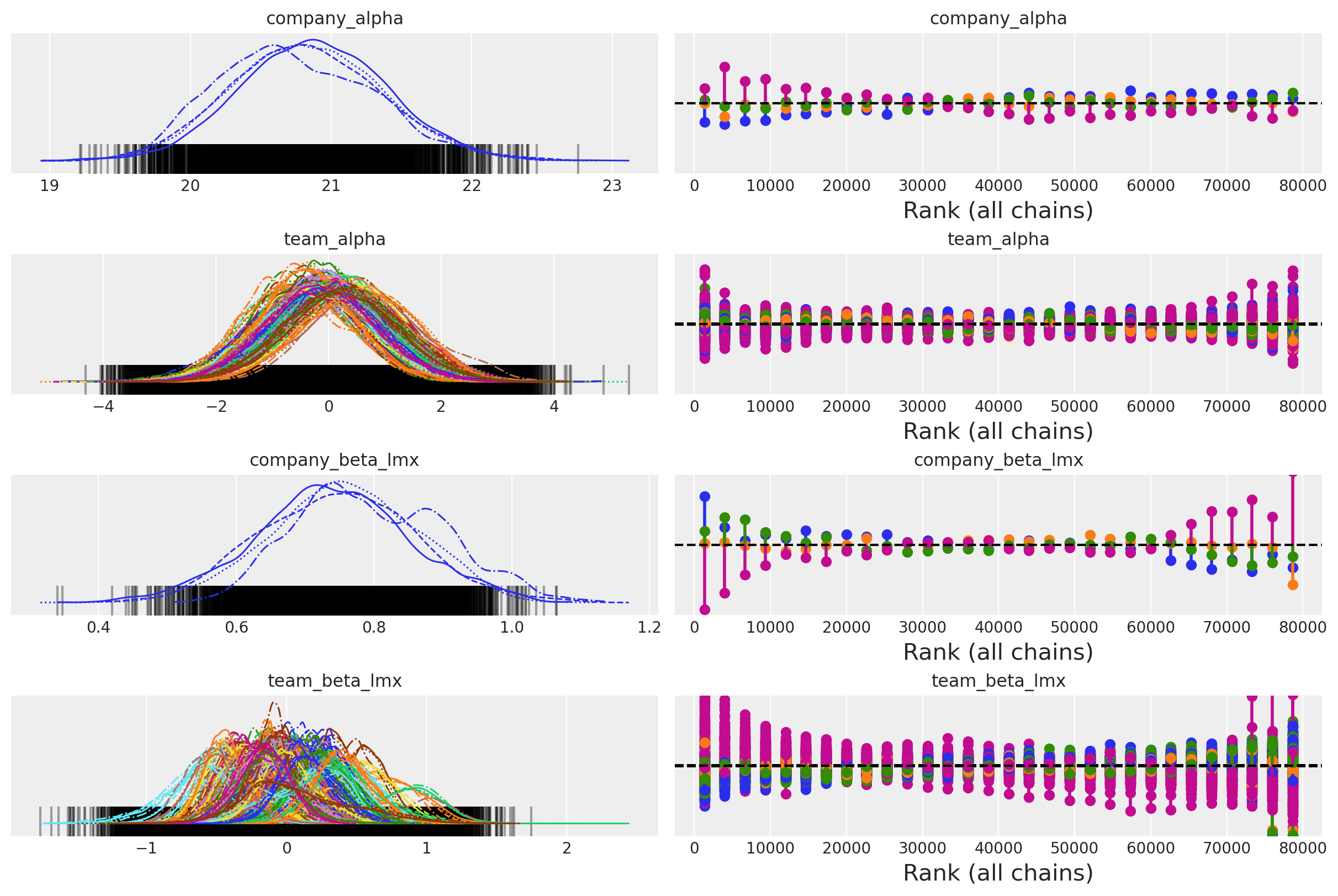
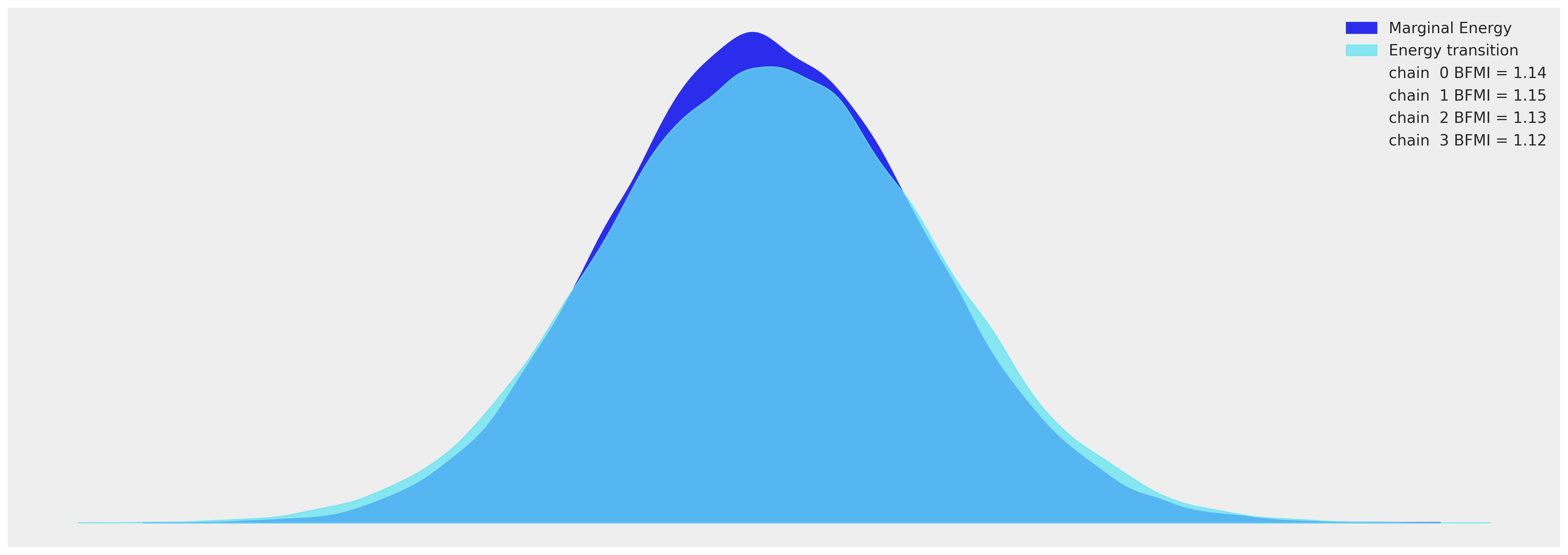
一些收敛性检查#
az.plot_trace(
idata_hierarchical,
var_names=["company_alpha", "team_alpha", "company_beta_lmx", "team_beta_lmx"],
kind="rank_vlines",
);
az.plot_energy(idata_hierarchical, figsize=(20, 7));
检查模型拟合#
summary = az.summary(
idata_hierarchical,
var_names=[
"company_alpha",
"team_alpha",
"company_beta_lmx",
"company_beta_male",
"team_beta_lmx",
],
)
summary
| mean | sd | hdi_3% | hdi_97% | mcse_mean | mcse_sd | ess_bulk | ess_tail | r_hat | |
|---|---|---|---|---|---|---|---|---|---|
| company_alpha | 20.818 | 0.545 | 19.806 | 21.840 | 0.029 | 0.020 | 358.0 | 1316.0 | 1.02 |
| team_alpha[1] | -0.214 | 0.955 | -1.975 | 1.604 | 0.030 | 0.021 | 1043.0 | 2031.0 | 1.00 |
| team_alpha[2] | -0.067 | 0.995 | -1.975 | 1.772 | 0.026 | 0.018 | 1496.0 | 2572.0 | 1.00 |
| team_alpha[3] | -0.568 | 0.931 | -2.271 | 1.250 | 0.027 | 0.019 | 1144.0 | 2135.0 | 1.00 |
| team_alpha[4] | -0.228 | 0.993 | -2.085 | 1.630 | 0.025 | 0.018 | 1552.0 | 4305.0 | 1.00 |
| ... | ... | ... | ... | ... | ... | ... | ... | ... | ... |
| team_beta_lmx[101] | 0.157 | 0.207 | -0.226 | 0.550 | 0.010 | 0.007 | 436.0 | 872.0 | 1.01 |
| team_beta_lmx[102] | 0.407 | 0.198 | 0.042 | 0.785 | 0.011 | 0.008 | 338.0 | 876.0 | 1.01 |
| team_beta_lmx[103] | -0.146 | 0.213 | -0.549 | 0.253 | 0.014 | 0.010 | 215.0 | 835.0 | 1.03 |
| team_beta_lmx[104] | -0.167 | 0.187 | -0.517 | 0.186 | 0.010 | 0.007 | 338.0 | 1346.0 | 1.01 |
| team_beta_lmx[105] | 0.071 | 0.393 | -0.562 | 0.902 | 0.021 | 0.015 | 390.0 | 476.0 | 1.01 |
213 行 × 9 列
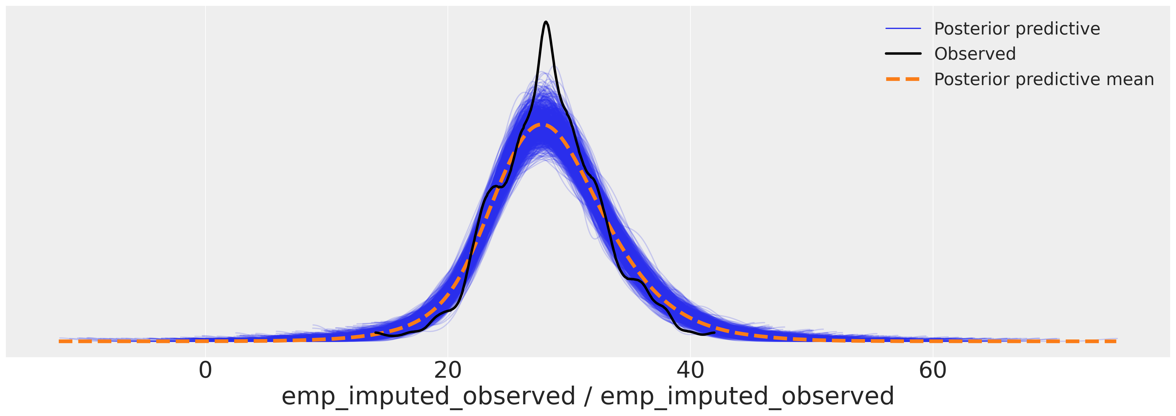
az.plot_ppc(
idata_hierarchical, var_names=["emp_imputed_observed"], figsize=(20, 7), num_pp_samples=1000
)
<AxesSubplot: xlabel='emp_imputed_observed / emp_imputed_observed'>
插补的异质性模式#
正如我们在考虑因果推断问题时关注局部因素的混杂影响一样,在进行插补时也需要这样做。我们在这里展示了一些团队特定的截距项,这些截距项表明,属于某个特定团队可能会使你的授权高于或低于公司级别截距项的总体平均值。这些环境的地方效应正是我们在插补缺失值时所要考虑的。
ax = az.plot_forest(
idata_hierarchical,
var_names=["team_beta_lmx"],
coords={"team": [1, 20, 22, 30, 50, 70, 76, 80, 100]},
figsize=(20, 15),
kind="ridgeplot",
combined=True,
ridgeplot_alpha=0.4,
hdi_prob=True,
)
ax[0].axvline(0)
ax[0].set_title("Team Contribution to the marginal effect of LMX on Empowerment", fontsize=20);
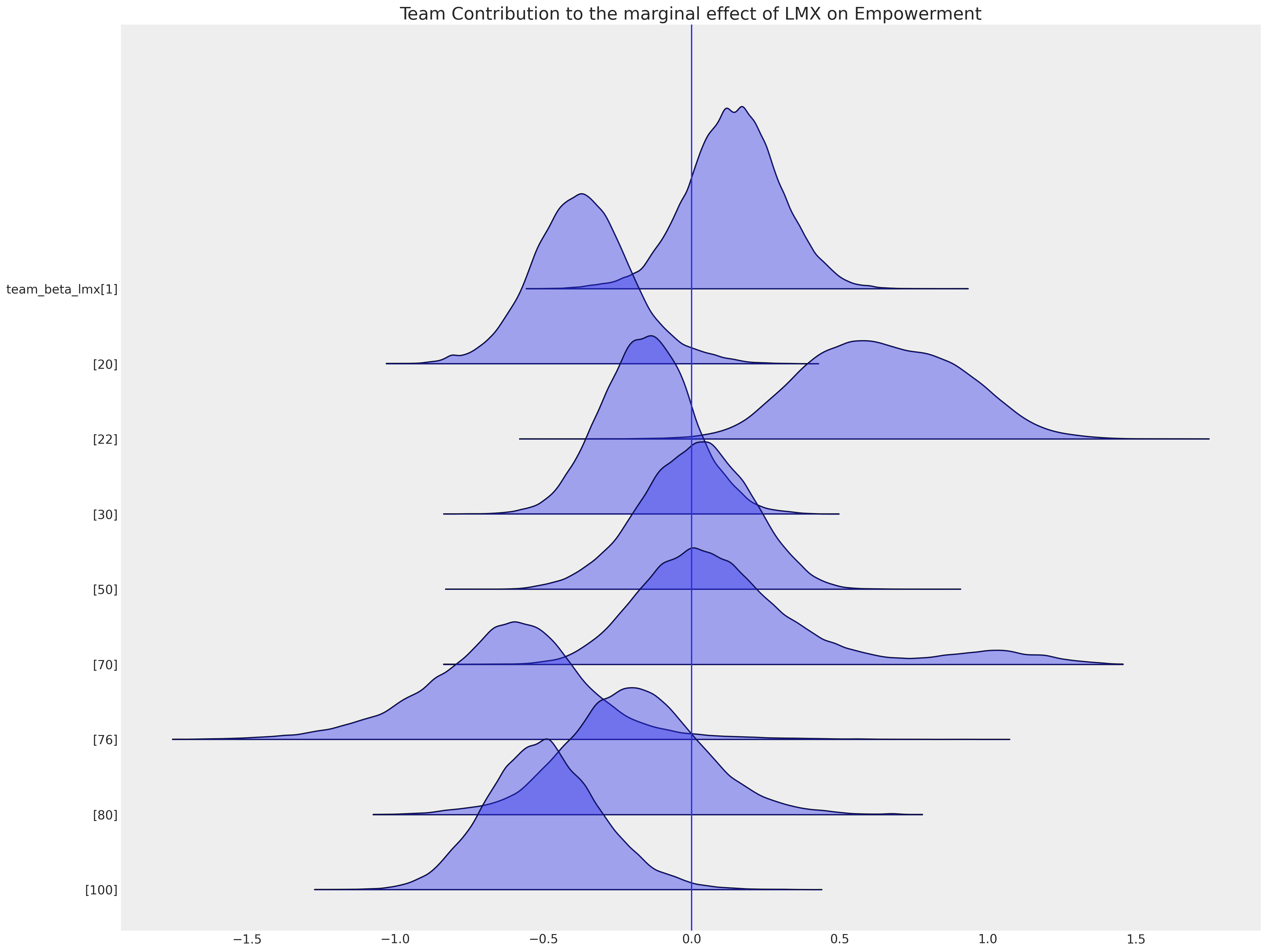
捕捉这种局部变化的能力也会影响插补值的模式。
imputed_data = df_employee[["lmx", "empower", "climate"]]
imputed_lmx = az.extract(idata_hierarchical, group="posterior_predictive", num_samples=1000)[
"lmx_pred"
].mean(axis=1)
mask = imputed_data["lmx"].isnull()
imputed_data.loc[mask, "lmx"] = imputed_lmx.values[imputed_data[mask].index]
imputed_emp = az.extract(idata_hierarchical, group="posterior_predictive", num_samples=1000)[
"emp_imputed"
].mean(axis=1)
mask = imputed_data["empower"].isnull()
imputed_data.loc[mask, "empower"] = imputed_emp.values[imputed_data[mask].index]
imputed_data.columns = ["imputed_" + col for col in imputed_data.columns]
joined = pd.concat([imputed_data, df_employee], axis=1)
joined["check"] = np.where(joined["empower"].isnull(), 1, 0)
mosaic = """AAAABB"""
fig, axs = plt.subplot_mosaic(mosaic, sharex=False, figsize=(20, 7))
axs = [axs[k] for k in axs.keys()]
axs[0].scatter(
joined["imputed_lmx"],
joined["imputed_empower"],
c=joined["check"],
cmap=cm.winter,
ec="black",
s=40,
)
z = multivariate_normal([10, joined["imputed_empower"].mean()], [[8.9, 5.4], [5.4, 19]]).pdf(
joined[["imputed_lmx", "imputed_empower"]]
)
axs[0].tricontour(joined["imputed_lmx"], joined["imputed_empower"], z)
axs[1].hist(joined["imputed_empower"], ec="black", label="Imputed", color="limegreen", bins=30)
axs[1].hist(joined["empower"], ec="black", label="observed", color="blue", bins=30)
axs[1].set_title("Empowerment Distributions Imputed \n with Team Informed Estimates", fontsize=20)
axs[0].set_xlabel("Leader Member Exchange - LMX")
axs[0].set_ylabel("Empowerment")
axs[0].set_title("Empowerment Imputed \n with Team Informed Estimates", fontsize=20)
axs[1].legend();
/var/folders/99/gp2xl6x513s0tvl3cx79zf7m0000gn/T/ipykernel_96943/3267370214.py:7: SettingWithCopyWarning:
A value is trying to be set on a copy of a slice from a DataFrame
See the caveats in the documentation: https://pandas.pydata.org/pandas-docs/stable/user_guide/indexing.html#returning-a-view-versus-a-copy
imputed_data.loc[mask, "lmx"] = imputed_lmx.values[imputed_data[mask].index]
/var/folders/99/gp2xl6x513s0tvl3cx79zf7m0000gn/T/ipykernel_96943/3267370214.py:13: SettingWithCopyWarning:
A value is trying to be set on a copy of a slice from a DataFrame
See the caveats in the documentation: https://pandas.pydata.org/pandas-docs/stable/user_guide/indexing.html#returning-a-view-versus-a-copy
imputed_data.loc[mask, "empower"] = imputed_emp.values[imputed_data[mask].index]
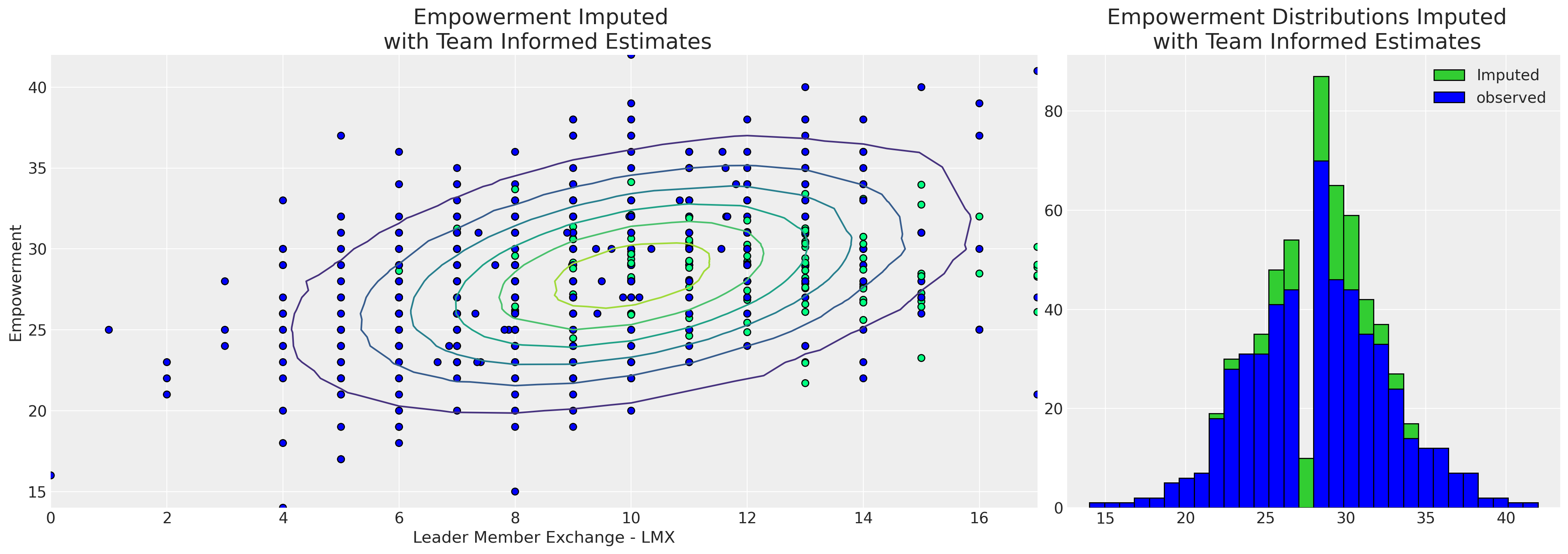
从层次模型可以清楚地看出,团队特定信息使我们能够根据lmx和male推算出更广泛范围的授权值,并且分布更广。由于所有的政治都是地方性的,并且后一种模型是根据每个员工的工作条件来构建的,因此这一点更具说服力。因此,我们的层次模型能够对缺失报告的可能授权值提供更细致的看法。层次插补模型通过两种方式“借用信息”:(i) 个体团队估计值向全局估计值靠拢,以及 (ii) 缺失值根据我们对团队动态的衡量进行插补。
结论#
我们已经看到了多种处理缺失数据的方法。我们专注于一个例子,其中缺失数据的原因并不明显,因为不同的员工可能会有不同的原因来低估他们与管理层的关系。然而,这里应用的技术是非常通用的。
多元正态逼近在许多情况下出奇地有效,但更前沿的方法是链式方程的顺序指定。这里的贝叶斯方法是最先进的,因为我们可以在我们的插补方程中自由使用比简单回归模型更复杂的模型。对于每个方程,我们可以自由选择似然项和我们在采样分布上允许的先验。我们还可以添加层次结构,以尊重我们数据中的自然聚类,只要它们限制了缺失数据的模式。
这一点很重要——贝叶斯方法的灵活性可以根据我们对数据缺失原因的理论的适当复杂性进行调整。类似的考虑也适用于反事实推理中涉及的估计程序。我们对数据缺失原因(为什么世界是这样的,而不是另一种方式)的理论越完善,我们就越需要一个灵活的建模框架来捕捉理论的细微差别。贝叶斯建模是理论构建和评估这一循环的绝佳工具。
参考资料#
Craig Enders K. 应用缺失数据分析。The Guilford Press, 2022.
水印#
%load_ext watermark
%watermark -n -u -v -iv -w -p pytensor
Last updated: Thu Feb 02 2023
Python implementation: CPython
Python version : 3.11.0
IPython version : 8.8.0
pytensor: 2.8.11
sys : 3.11.0 | packaged by conda-forge | (main, Jan 15 2023, 05:44:48) [Clang 14.0.6 ]
pytensor : 2.8.11
scipy : 1.10.0
pymc : 5.0.1
numpy : 1.24.1
matplotlib: 3.6.3
arviz : 0.14.0
pandas : 1.5.2
Watermark: 2.3.1