


使用“黑箱”似然函数#
注意
有一个相关示例讨论了如何使用在JAX中实现的似然函数
import arviz as az
import matplotlib.pyplot as plt
import numpy as np
import pymc as pm
import pytensor
import pytensor.tensor as pt

from pytensor.graph import Apply, Op
from scipy.optimize import approx_fprime

print(f"Running on PyMC v{pm.__version__}")
Running on PyMC v5.10.3
%config InlineBackend.figure_format = 'retina'
az.style.use("arviz-darkgrid")
介绍#
PyMC 是一个用于进行贝叶斯推断和参数估计的强大工具。它有许多 内置的概率分布,您可以使用它们为您的特定模型设置先验和似然函数。您甚至可以创建自己的 自定义分布,并使用 PyTensor 操作定义自定义 logp,或者从生成图自动推断。
尽管有这些“内置电池”,您可能仍然发现自己需要处理依赖于复杂外部代码的模型函数或概率分布,这些代码您无法避免使用。这些代码不太可能与PyMC使用的抽象PyTensor变量兼容:PyMC 和 PyTensor。
import pymc as pm
from external_module import my_external_func  # your external function!

# set up your model
with pm.Model():
    # your external function takes two parameters, a and b, with Uniform priors
    a = pm.Uniform('a', lower=0., upper=1.)
    b = pm.Uniform('b', lower=0., upper=1.)

    m = my_external_func(a, b)  # <--- this is not going to work!
另一个问题是,如果你想使用基于梯度的步长采样器,如NUTS和哈密顿蒙特卡洛,那么你的模型/似然函数需要定义一个梯度。如果你的模型是定义为一组 PyTensor 操作符,那么这不会有问题——内部它将能够进行自动微分——但如果你的模型本质上是一个“黑箱”,那么你不一定知道梯度是什么。
定义一个PyMC可以使用的模型/似然函数,并调用您的“黑盒”函数是可能的,但这依赖于创建一个自定义的PyTensor Op。希望这是一个清晰的描述,说明如何做到这一点,包括一种编写梯度函数的方法,该方法可能具有普遍适用性。
在下面的示例中,我们使用numpy创建了一个非常简单的线性模型和对数似然函数。
def my_model(m, c, x):
    return m * x + c


def my_loglike(m, c, sigma, x, data):
    # We fail explicitly if inputs are not numerical types for the sake of this tutorial
    # As defined, my_loglike would actually work fine with PyTensor variables!
    for param in (m, c, sigma, x, data):
        if not isinstance(param, (float, np.ndarray)):
            raise TypeError(f"Invalid input type to loglike: {type(param)}")
    model = my_model(m, c, x)
    return -0.5 * ((data - model) / sigma) ** 2 - np.log(np.sqrt(2 * np.pi)) - np.log(sigma)
现在,按照目前的情况,如果我们想从这个对数似然函数中采样,使用某些先验分布作为模型参数(斜率和截距),使用PyMC,我们可能会尝试这样做(使用pymc.CustomDist 或 pymc.Potential):
import pymc as pm

# create/read in our "data" (I'll show this in the real example below)
x = ...
sigma = ...
data = ...

with pm.Model():
    # set priors on model gradient and y-intercept
    m = pm.Uniform('m', lower=-10., upper=10.)
    c = pm.Uniform('c', lower=-10., upper=10.)

    # create custom distribution
    pm.CustomDist('likelihood', m, c, sigma, x, observed=data, logp=my_loglike)

    # sample from the distribution
    trace = pm.sample(1000)
但是,当黑箱函数不接受 PyTensor 张量对象作为输入时,这可能会导致错误。
因此,我们实际上需要做的是创建一个PyTensor Op。这将是一个新的类,它包装了我们的对数似然函数,同时遵守 PyTensor API 契约。我们将在下面这样做,最初不定义 Op 的 grad()。
提示
根据您的应用程序,您可能只需要封装一个自定义的对数似然函数或整个模型的一部分(例如,使用像mpmath这样的高级库计算无限级数和的函数),然后可以将其与其他PyMC分布和PyTensor操作链接起来,以定义您的整个模型。这里有一个权衡,通常情况下,您从黑箱中省略的越多,您可能从PyTensor的重写和优化中受益越多。我们建议您始终尝试在PyMC和PyTensor中定义整个模型,并且仅在严格必要时使用黑箱。
PyTensor 操作无梯度#
操作定义#
# define a pytensor Op for our likelihood function


class LogLike(Op):
    def make_node(self, m, c, sigma, x, data) -> Apply:
        # Convert inputs to tensor variables
        m = pt.as_tensor(m)
        c = pt.as_tensor(c)
        sigma = pt.as_tensor(sigma)
        x = pt.as_tensor(x)
        data = pt.as_tensor(data)

        inputs = [m, c, sigma, x, data]
        # Define output type, in our case a vector of likelihoods
        # with the same dimensions and same data type as data
        # If data must always be a vector, we could have hard-coded
        # outputs = [pt.vector()]
        outputs = [data.type()]

        # Apply is an object that combines inputs, outputs and an Op (self)
        return Apply(self, inputs, outputs)

    def perform(self, node: Apply, inputs: list[np.ndarray], outputs: list[list[None]]) -> None:
        # This is the method that compute numerical output
        # given numerical inputs. Everything here is numpy arrays
        m, c, sigma, x, data = inputs  # this will contain my variables

        # call our numpy log-likelihood function
        loglike_eval = my_loglike(m, c, sigma, x, data)

        # Save the result in the outputs list provided by PyTensor
        # There is one list per output, each containing another list
        # pre-populated with a `None` where the result should be saved.
        outputs[0][0] = np.asarray(loglike_eval)
# set up our data
N = 10  # number of data points
sigma = 1.0  # standard deviation of noise
x = np.linspace(0.0, 9.0, N)

mtrue = 0.4  # true gradient
ctrue = 3.0  # true y-intercept

truemodel = my_model(mtrue, ctrue, x)

# make data
rng = np.random.default_rng(716743)
data = sigma * rng.normal(size=N) + truemodel
现在我们有了一些数据,我们初始化实际的Op并尝试使用它。
# create our Op
loglike_op = LogLike()

test_out = loglike_op(mtrue, ctrue, sigma, x, data)
pytensor.dprint 打印 PyTensor 图的文本表示。
我们可以看到我们的变量是 LogLike Op 的输出,并且具有 pt.vector(float64, shape=(10,)) 的类型。
我们还可以看到五个常量输入及其类型。
pytensor.dprint(test_out, print_type=True)
LogLike [id A] <Vector(float64, shape=(10,))>
 ├─ 0.4 [id B] <Scalar(float64, shape=())>
 ├─ 3.0 [id C] <Scalar(float32, shape=())>
 ├─ 1.0 [id D] <Scalar(float32, shape=())>
 ├─ [0. 1. 2. ... 7. 8. 9.] [id E] <Vector(float64, shape=(10,))>
 └─ [2.3876939 ... .56436476] [id F] <Vector(float64, shape=(10,))>
<ipykernel.iostream.OutStream at 0x7f462db44100>
因为所有输入都是常量,我们可以使用方便的 eval 方法来评估输出
test_out.eval()
array([-1.1063979 , -0.92587551, -1.34602737, -0.91918325, -1.72027674,
       -1.2816813 , -0.91895074, -1.02783982, -1.68422175, -1.45520871])
我们可以确认这返回了我们期望的结果
my_loglike(mtrue, ctrue, sigma, x, data)
array([-1.1063979 , -0.92587551, -1.34602737, -0.91918325, -1.72027674,
       -1.2816813 , -0.91895074, -1.02783982, -1.68422175, -1.45520871])
模型定义#
现在,让我们使用这个Op来重复上面展示的例子。为此,我们创建一些包含直线和附加高斯噪声(均值为零,标准差为sigma)的数据。为了简单起见,我们在斜率和y截距上设置了Uniform先验分布。由于我们没有设置Op的grad()方法,PyMC将无法使用基于梯度的采样器,因此将回退到使用pymc.Slice采样器。
def custom_dist_loglike(data, m, c, sigma, x):
    # data, or observed is always passed as the first input of CustomDist
    return loglike_op(m, c, sigma, x, data)


# use PyMC to sampler from log-likelihood
with pm.Model() as no_grad_model:
    # uniform priors on m and c
    m = pm.Uniform("m", lower=-10.0, upper=10.0, initval=mtrue)
    c = pm.Uniform("c", lower=-10.0, upper=10.0, initval=ctrue)

    # use a CustomDist with a custom logp function
    likelihood = pm.CustomDist(
        "likelihood", m, c, sigma, x, observed=data, logp=custom_dist_loglike
    )
在我们采样之前,我们可以检查模型logp是否正确(并且没有错误被抛出)。
我们需要一个点来评估logp,我们可以通过initial_point方法获得。
这将是我们在模型中定义的转换后的初始值。
ip = no_grad_model.initial_point()
ip
{'m_interval__': array(0.08004271), 'c_interval__': array(0.61903921)}
我们应该得到与我们手动测试时完全相同的值!
no_grad_model.compile_logp(vars=[likelihood], sum=False)(ip)
[array([-1.1063979 , -0.92587551, -1.34602737, -0.91918325, -1.72027674,
        -1.2816813 , -0.91895074, -1.02783982, -1.68422175, -1.45520871])]
我们也可以再次确认,如果我们尝试提取模型关于对数概率(我们称之为dlogp)的梯度,PyMC将会报错。
try:
    no_grad_model.compile_dlogp()
except Exception as exc:
    print(type(exc))
<class 'NotImplementedError'>
最后,让我们来采样!
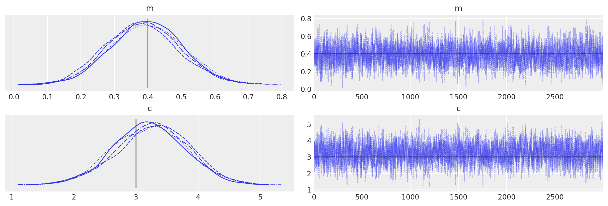
with no_grad_model:
    # Use custom number of draws to replace the HMC based defaults
    idata_no_grad = pm.sample(3000, tune=1000)

# plot the traces
az.plot_trace(idata_no_grad, lines=[("m", {}, mtrue), ("c", {}, ctrue)]);
Multiprocess sampling (4 chains in 4 jobs)
CompoundStep
>Slice: [m]
>Slice: [c]
Sampling 4 chains for 1_000 tune and 3_000 draw iterations (4_000 + 12_000 draws total) took 4 seconds.
PyTensor Op with gradients#
如果我们想使用NUTS或HMC呢?如果我们知道模型/似然函数的解析导数,那么我们可以使用现有的PyTensor操作向Op添加一个grad()。
但是,如果我们不知道解析形式怎么办?如果我们的模型/似然函数是在一个提供自动微分功能的框架中实现的(就像 PyTensor 那样),那么我们可以重用它们的功能。这个 相关示例 展示了在使用 JAX 函数时如何实现这一点。
如果我们的模型/似然性确实是一个“黑箱”,那么我们可以尝试使用近似方法,如有限差分来找到梯度。我们通过方便的SciPy approx_fprime()函数来说明这种方法。
注意
有限差分很少被推荐作为计算梯度的一种方法。它们在实际应用中可能太慢或不稳定。我们建议您仅在万不得已时使用它们。
操作定义#
def finite_differences_loglike(m, c, sigma, x, data, eps=1e-7):
    """
    Calculate the partial derivatives of a function at a set of values. The
    derivatives are calculated using scipy approx_fprime function.

    Parameters
    ----------
    m, c: array_like
        The parameters of the function for which we wish to define partial derivatives
    x, data, sigma:
        Observed variables as we have been using so far


    Returns
    -------
    grad_wrt_m: array_like
        Partial derivative wrt to the m parameter
    grad_wrt_c: array_like
        Partial derivative wrt to the c parameter
    """

    def inner_func(mc, sigma, x, data):
        return my_loglike(*mc, sigma, x, data)

    grad_wrt_mc = approx_fprime([m, c], inner_func, [eps, eps], sigma, x, data)

    return grad_wrt_mc[:, 0], grad_wrt_mc[:, 1]
finite_differences_loglike(mtrue, ctrue, sigma, x, data)
(array([ 0.        , -0.11778783,  1.84843447, -0.06637035,  5.06387346,
         4.2587707 ,  0.02964459, -3.2668551 ,  9.89728189, -9.32072126]),
 array([-0.61230613, -0.11778783,  0.92421729, -0.02212335,  1.26596852,
         0.85175434,  0.00494102, -0.46669328,  1.23716059, -1.0356353 ]))
所以,现在我们可以用一个grad()方法重新定义我们的Op,对吧?
这并不那么简单!grad() 方法本身要求其输入是 PyTensor 张量变量,而我们的 gradients 函数,就像我们的 my_loglike 函数一样,需要一个浮点值列表。因此,我们需要定义另一个计算梯度的 Op。下面,我定义了一个新的 LogLike Op 版本,这次叫做 LogLikeWithGrad,它有一个 grad() 方法。接下来是另一个叫做 LogLikeGrad 的 Op,当它被调用时,传入一个 PyTensor 张量变量向量,返回另一个向量,这些值是我们的对数似然函数在这些值处的梯度(即 雅可比矩阵)。请注意,grad() 方法本身并不直接返回梯度,而是返回 雅可比向量积。
# define a pytensor Op for our likelihood function


class LogLikeWithGrad(Op):
    def make_node(self, m, c, sigma, x, data) -> Apply:
        # Same as before
        m = pt.as_tensor(m)
        c = pt.as_tensor(c)
        sigma = pt.as_tensor(sigma)
        x = pt.as_tensor(x)
        data = pt.as_tensor(data)

        inputs = [m, c, sigma, x, data]
        outputs = [data.type()]
        return Apply(self, inputs, outputs)

    def perform(self, node: Apply, inputs: list[np.ndarray], outputs: list[list[None]]) -> None:
        # Same as before
        m, c, sigma, x, data = inputs  # this will contain my variables
        loglike_eval = my_loglike(m, c, sigma, x, data)
        outputs[0][0] = np.asarray(loglike_eval)

    def grad(
        self, inputs: list[pt.TensorVariable], g: list[pt.TensorVariable]
    ) -> list[pt.TensorVariable]:
        # NEW!
        # the method that calculates the gradients - it actually returns the vector-Jacobian product
        m, c, sigma, x, data = inputs

        # Our gradient expression assumes these are scalar parameters
        if m.type.ndim != 0 or c.type.ndim != 0:
            raise NotImplementedError("Gradient only implemented for scalar m and c")

        grad_wrt_m, grad_wrt_c = loglikegrad_op(m, c, sigma, x, data)

        # out_grad is a tensor of gradients of the Op outputs wrt to the function cost
        [out_grad] = g
        return [
            pt.sum(out_grad * grad_wrt_m),
            pt.sum(out_grad * grad_wrt_c),
            # We did not implement gradients wrt to the last 3 inputs
            # This won't be a problem for sampling, as those are constants in our model
            pytensor.gradient.grad_not_implemented(self, 2, sigma),
            pytensor.gradient.grad_not_implemented(self, 3, x),
            pytensor.gradient.grad_not_implemented(self, 4, data),
        ]


class LogLikeGrad(Op):
    def make_node(self, m, c, sigma, x, data) -> Apply:
        m = pt.as_tensor(m)
        c = pt.as_tensor(c)
        sigma = pt.as_tensor(sigma)
        x = pt.as_tensor(x)
        data = pt.as_tensor(data)

        inputs = [m, c, sigma, x, data]
        # There are two outputs with the same type as data,
        # for the partial derivatives wrt to m, c
        outputs = [data.type(), data.type()]

        return Apply(self, inputs, outputs)

    def perform(self, node: Apply, inputs: list[np.ndarray], outputs: list[list[None]]) -> None:
        m, c, sigma, x, data = inputs

        # calculate gradients
        grad_wrt_m, grad_wrt_c = finite_differences_loglike(m, c, sigma, x, data)

        outputs[0][0] = grad_wrt_m
        outputs[1][0] = grad_wrt_c


# Initalize the Ops
loglikewithgrad_op = LogLikeWithGrad()
loglikegrad_op = LogLikeGrad()
在我们回到模型之前,我们应该测试梯度是否正常工作。
我们不会直接评估 loglikegrad_op,而是使用 PyMC 最终会使用的相同 PyTensor grad 机制,以确保没有意外。
为此,我们将为 m 和 c 提供符号输入(在 PyMC 模型中,它们将是随机变量)。
由于我们的loglike Op也是新的,让我们确保它的输出仍然是正确的。我们仍然可以使用eval,但由于我们有两个非常量输入,我们需要为这些输入提供值。
eval_out = out.eval({m: mtrue, c: ctrue})
print(eval_out)
assert np.allclose(eval_out, my_loglike(mtrue, ctrue, sigma, x, data))
[-1.1063979  -0.92587551 -1.34602737 -0.91918325 -1.72027674 -1.2816813
 -0.91895074 -1.02783982 -1.68422175 -1.45520871]
如果你感兴趣,你可以看看梯度计算图是什么样子的,但它有点混乱。
你可以看到,LogLikeWithGrad 和 LogLikeGrad 都如预期显示
grad_wrt_m, grad_wrt_c = pytensor.grad(out.sum(), wrt=[m, c])
pytensor.dprint([grad_wrt_m], print_type=True)
Sum{axes=None} [id A] <Scalar(float64, shape=())>
 └─ Mul [id B] <Vector(float64, shape=(10,))>
    ├─ Second [id C] <Vector(float64, shape=(10,))>
    │  ├─ LogLikeWithGrad [id D] <Vector(float64, shape=(10,))>
    │  │  ├─ m [id E] <Scalar(float64, shape=())>
    │  │  ├─ c [id F] <Scalar(float64, shape=())>
    │  │  ├─ 1.0 [id G] <Scalar(float32, shape=())>
    │  │  ├─ [0. 1. 2. ... 7. 8. 9.] [id H] <Vector(float64, shape=(10,))>
    │  │  └─ [2.3876939 ... .56436476] [id I] <Vector(float64, shape=(10,))>
    │  └─ ExpandDims{axis=0} [id J] <Vector(float64, shape=(1,))>
    │     └─ Second [id K] <Scalar(float64, shape=())>
    │        ├─ Sum{axes=None} [id L] <Scalar(float64, shape=())>
    │        │  └─ LogLikeWithGrad [id D] <Vector(float64, shape=(10,))>
    │        │     └─ ···
    │        └─ 1.0 [id M] <Scalar(float64, shape=())>
    └─ LogLikeGrad.0 [id N] <Vector(float64, shape=(10,))>
       ├─ m [id E] <Scalar(float64, shape=())>
       ├─ c [id F] <Scalar(float64, shape=())>
       ├─ 1.0 [id G] <Scalar(float32, shape=())>
       ├─ [0. 1. 2. ... 7. 8. 9.] [id H] <Vector(float64, shape=(10,))>
       └─ [2.3876939 ... .56436476] [id I] <Vector(float64, shape=(10,))>
<ipykernel.iostream.OutStream at 0x7f462db44100>
确认我们正确实现梯度的最佳方法是使用 PyTensor 的 verify_grad 工具
def test_fn(m, c):
    return loglikewithgrad_op(m, c, sigma, x, data)


# This raises an error if the gradient output is not within a given tolerance
pytensor.gradient.verify_grad(test_fn, pt=[mtrue, ctrue], rng=np.random.default_rng(123))
模型定义#
现在,让我们用新的“grad”操作重新运行PyMC。这次它将能够自动使用NUTS。
def custom_dist_loglike(data, m, c, sigma, x):
    # data, or observed is always passed as the first input of CustomDist
    return loglikewithgrad_op(m, c, sigma, x, data)


# use PyMC to sampler from log-likelihood
with pm.Model() as grad_model:
    # uniform priors on m and c
    m = pm.Uniform("m", lower=-10.0, upper=10.0)
    c = pm.Uniform("c", lower=-10.0, upper=10.0)

    # use a CustomDist with a custom logp function
    likelihood = pm.CustomDist(
        "likelihood", m, c, sigma, x, observed=data, logp=custom_dist_loglike
    )
对数似然值不应该发生变化。
grad_model.compile_logp(vars=[likelihood], sum=False)(ip)
[array([-1.1063979 , -0.92587551, -1.34602737, -0.91918325, -1.72027674,
        -1.2816813 , -0.91895074, -1.02783982, -1.68422175, -1.45520871])]
但这次我们应该能够评估 dlogp(关于 m 和 c)
grad_model.compile_dlogp()(ip)
array([41.52474277, 8.93420609])
因此,NUTS 现在将默认被选中
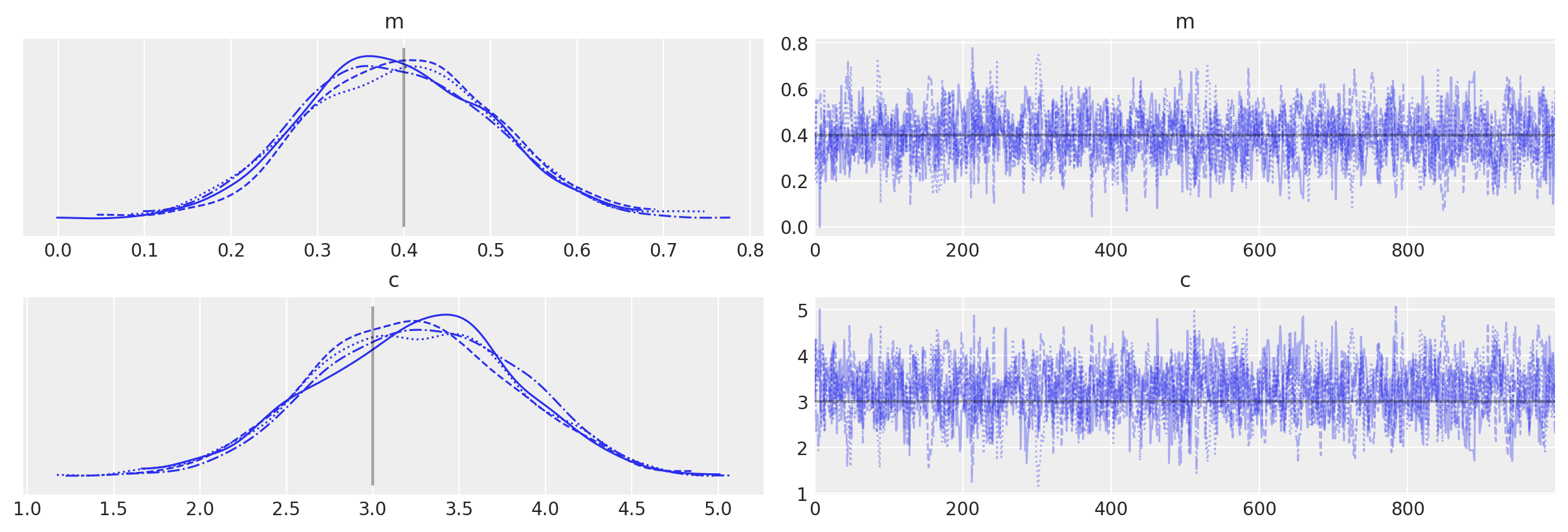
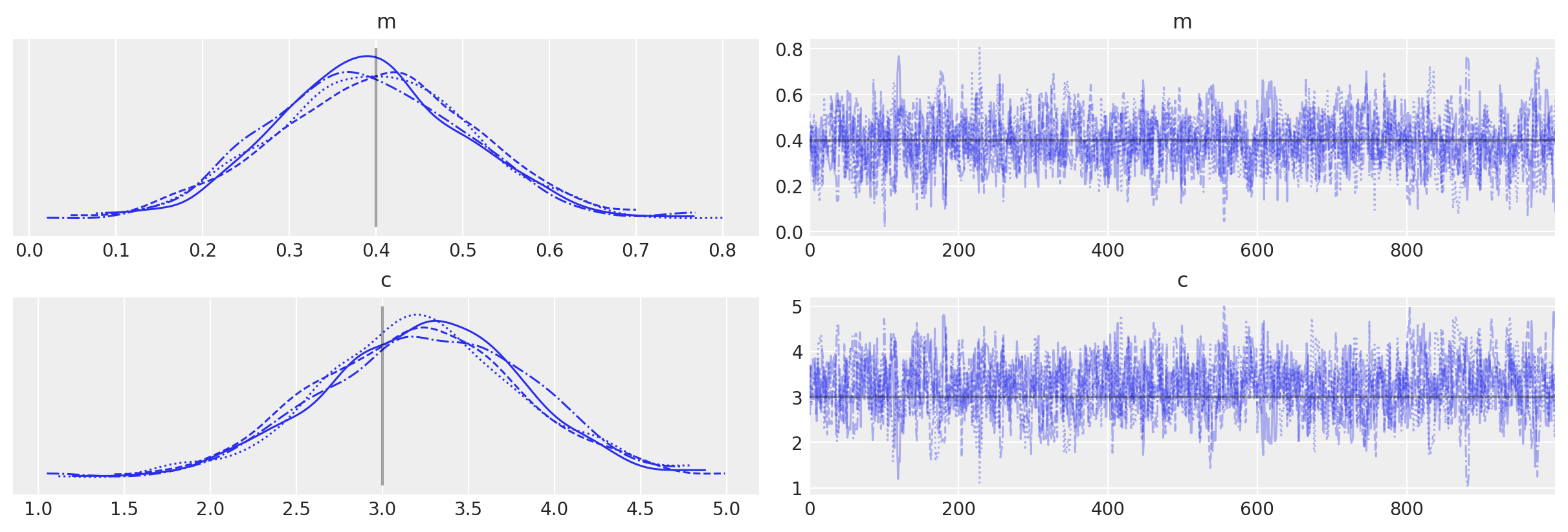
with grad_model:
    # Use custom number of draws to replace the HMC based defaults
    idata_grad = pm.sample()

# plot the traces
az.plot_trace(idata_grad, lines=[("m", {}, mtrue), ("c", {}, ctrue)]);
Auto-assigning NUTS sampler...
Initializing NUTS using jitter+adapt_diag...
Multiprocess sampling (4 chains in 4 jobs)
NUTS: [m, c]
Sampling 4 chains for 1_000 tune and 1_000 draw iterations (4_000 + 4_000 draws total) took 8 seconds.
与等效的PyMC分布的比较#
最后,为了检查事情是否如我们预期的那样工作,让我们完全使用PyMC分布来做同样的事情(因为在这个简单的例子中我们可以!)
with pm.Model() as pure_model:
    # uniform priors on m and c
    m = pm.Uniform("m", lower=-10.0, upper=10.0)
    c = pm.Uniform("c", lower=-10.0, upper=10.0)

    # use a Normal distribution
    likelihood = pm.Normal("likelihood", mu=(m * x + c), sigma=sigma, observed=data)
pure_model.compile_logp(vars=[likelihood], sum=False)(ip)
[array([-1.1063979 , -0.92587551, -1.34602737, -0.91918325, -1.72027674,
        -1.2816813 , -0.91895074, -1.02783982, -1.68422175, -1.45520871])]
pure_model.compile_dlogp()(ip)
array([41.52481384, 8.9342084 ])
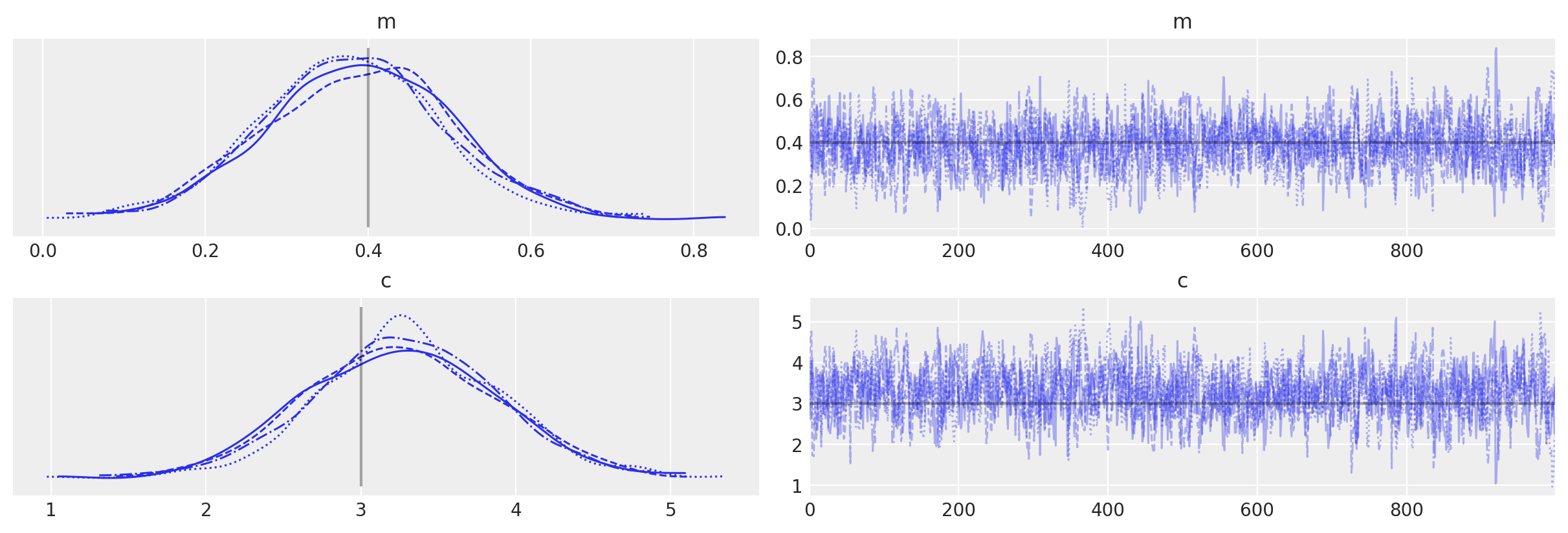
with pure_model:
    idata_pure = pm.sample()

# plot the traces
az.plot_trace(idata_pure, lines=[("m", {}, mtrue), ("c", {}, ctrue)]);
Auto-assigning NUTS sampler...
Initializing NUTS using jitter+adapt_diag...
Multiprocess sampling (4 chains in 4 jobs)
NUTS: [m, c]
Sampling 4 chains for 1_000 tune and 1_000 draw iterations (4_000 + 4_000 draws total) took 3 seconds.
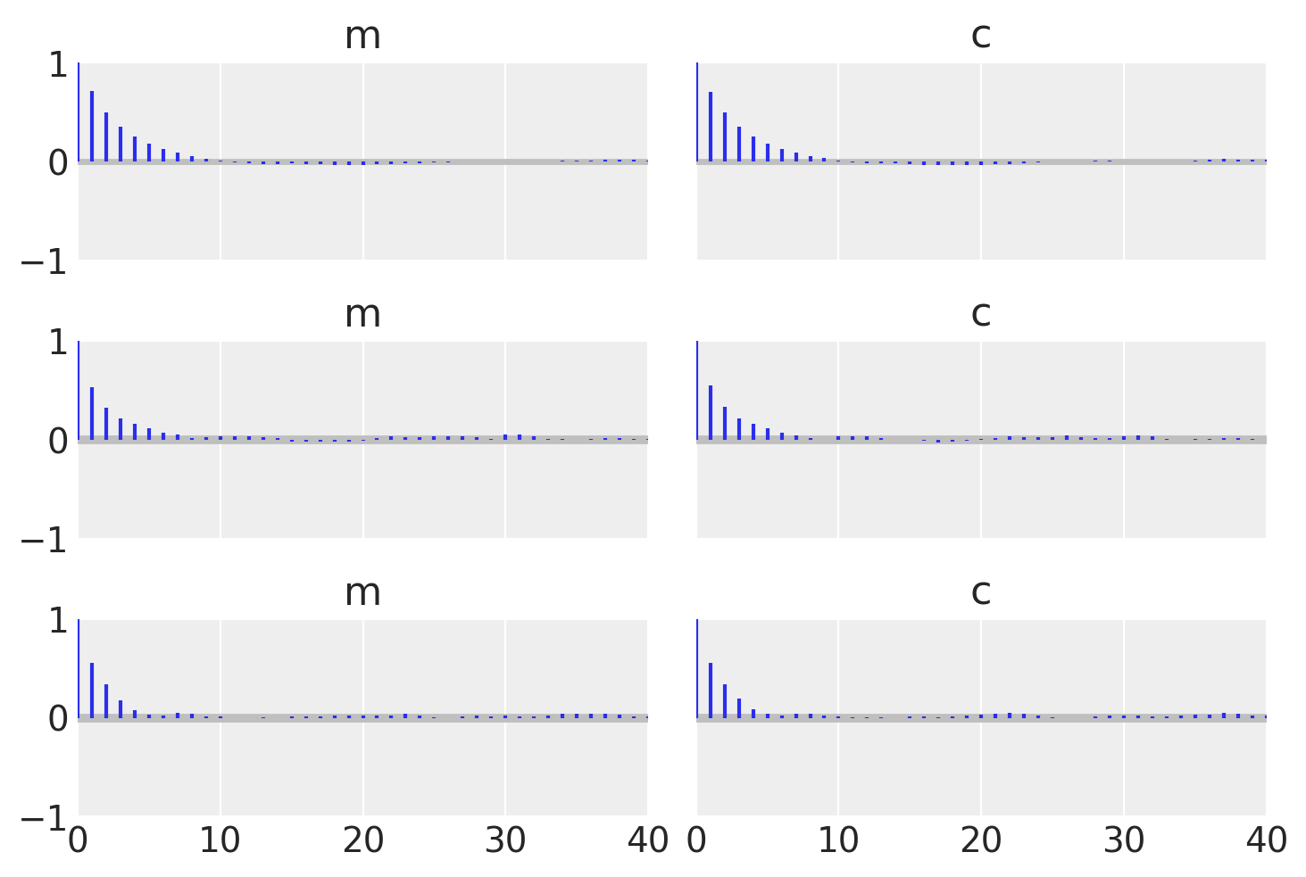
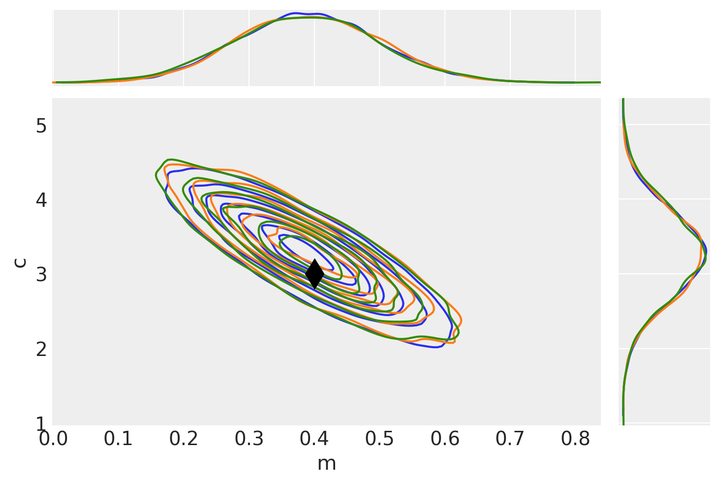
为了检查它们是否匹配,让我们将所有示例一起绘制,并找出自相关长度。
_, axes = plt.subplots(3, 2, sharex=True, sharey=True)
az.plot_autocorr(idata_no_grad, combined=True, ax=axes[0, :])
az.plot_autocorr(idata_grad, combined=True, ax=axes[1, :])
az.plot_autocorr(idata_pure, combined=True, ax=axes[2, :])
axes[2, 0].set_xlim(right=40);
# Plot no grad result (blue)
pair_kwargs = dict(
    kind="kde",
    marginals=True,
    reference_values={"m": mtrue, "c": ctrue},
    kde_kwargs={"contourf_kwargs": {"alpha": 0}, "contour_kwargs": {"colors": "C0"}},
    reference_values_kwargs={"color": "k", "ms": 15, "marker": "d"},
    marginal_kwargs={"color": "C0"},
)
ax = az.plot_pair(idata_no_grad, **pair_kwargs)

# Plot nuts+blackbox fit (orange)
pair_kwargs["kde_kwargs"]["contour_kwargs"]["colors"] = "C1"
pair_kwargs["marginal_kwargs"]["color"] = "C1"
az.plot_pair(idata_grad, **pair_kwargs, ax=ax)

# Plot pure pymc+nuts fit (green)
pair_kwargs["kde_kwargs"]["contour_kwargs"]["colors"] = "C2"
pair_kwargs["marginal_kwargs"]["color"] = "C2"
az.plot_pair(idata_pure, **pair_kwargs, ax=ax);
/home/ricardo/miniconda3/envs/pymc-examples/lib/python3.11/site-packages/arviz/plots/pairplot.py:232: FutureWarning: The return type of `Dataset.dims` will be changed to return a set of dimension names in future, in order to be more consistent with `DataArray.dims`. To access a mapping from dimension names to lengths, please use `Dataset.sizes`.
  gridsize = int(dataset.dims["draw"] ** 0.35)
使用势能而不是CustomDist#
在本节中,我们展示了如何使用pymc.Potential()来更直接地实现黑箱似然函数,而不是使用pymc.CustomDist。
更简单的接口是以使贝叶斯工作流的其它部分更加繁琐为代价的。例如,由于 pymc.Potential() 不能用于模型比较,因为 PyMC 不知道一个 Potential 项对应于先验、似然还是两者的混合。Potential 也没有前向采样的对应物,这对于先验和后验预测采样是必需的,而 pymc.CustomDist 接受 random 或 dist 函数用于此类场合。
with pm.Model() as potential_model:
    # uniform priors on m and c
    m = pm.Uniform("m", lower=-10.0, upper=10.0)
    c = pm.Uniform("c", lower=-10.0, upper=10.0)

    # use a Potential instead of a CustomDist
    pm.Potential("likelihood", loglikewithgrad_op(m, c, sigma, x, data))

    idata_potential = pm.sample()

# plot the traces
az.plot_trace(idata_potential, lines=[("m", {}, mtrue), ("c", {}, ctrue)]);
Auto-assigning NUTS sampler...
Initializing NUTS using jitter+adapt_diag...
Multiprocess sampling (4 chains in 4 jobs)
NUTS: [m, c]
Sampling 4 chains for 1_000 tune and 1_000 draw iterations (4_000 + 4_000 draws total) took 8 seconds.
水印#
%load_ext watermark
%watermark -n -u -v -iv -w -p xarray
Last updated: Wed Mar 13 2024

Python implementation: CPython
Python version       : 3.11.7
IPython version      : 8.21.0

xarray: 2024.1.1

arviz     : 0.17.0
pytensor  : 2.18.6
numpy     : 1.26.3
pymc      : 5.10.3
matplotlib: 3.8.2

Watermark: 2.4.3