离散变量的自动边缘化

PyMC非常适合用于对具有离散潜在变量的模型进行采样。但如果你坚持只使用NUTS采样器，你需要以某种方式消除离散变量。最好的方法是边缘化它们，这样你可以受益于Rao-Blackwell定理，并获得参数的较低方差估计。

形式上，这个论点是这样的，采样器可以理解为近似期望值 \(\mathbb{E}_{p(x, z)}[f(x, z)]\) 对于某个函数 \(f\) 相对于分布 \(p(x, z)\)。根据全期望定律，我们知道

\[ \mathbb{E}_{p(x, z)}[f(x, z)] = \mathbb{E}_{p(z)}\left[\mathbb{E}_{p(x \mid z)}\left[f(x, z)\right]\right] \]

令 \(g(z) = \mathbb{E}_{p(x \mid z)}\left[f(x, z)\right]\)，根据全变差定律，我们知道

\[ \mathbb{V}_{p(x, z)}[f(x, z)] = \mathbb{V}_{p(z)}[g(z)] + \mathbb{E}_{p(z)}\left[\mathbb{V}_{p(x \mid z)}\left[f(x, z)\right]\right] \]

因为期望值是针对方差计算的，所以它必须始终为正，因此我们知道

\[ \mathbb{V}_{p(x, z)}[f(x, z)] \geq \mathbb{V}_{p(z)}[g(z)] \]

直观地说，在模型中边缘化变量可以让您使用 \(g\) 而不是 \(f\)。这种较低的方差最直接体现在较低的蒙特卡罗标准误差（mcse），间接体现在通常较高的有效样本量（ESS）。

不幸的是，进行这种计算通常是繁琐且不直观的。幸运的是，pymc-experimental 现在支持自动完成这项工作！

import arviz as az
import matplotlib.pyplot as plt
import numpy as np
import pandas as pd
import pymc as pm
import pytensor.tensor as pt

import pymc_experimental as pmx

%config InlineBackend.figure_format = 'retina'  # high resolution figures
az.style.use("arviz-darkgrid")
rng = np.random.default_rng(32)

作为一个激励性的例子，考虑一个高斯混合模型

高斯混合模型

有两种方法可以指定相同的模型。一种是明确选择混合的方式。

mu = pt.as_tensor([-2.0, 2.0])

with pmx.MarginalModel() as explicit_mixture:
    idx = pm.Bernoulli("idx", 0.7)
    y = pm.Normal("y", mu=mu[idx], sigma=1.0)

plt.hist(pm.draw(y, draws=2000, random_seed=rng), bins=30, rwidth=0.9);

另一种方法是使用内置的 NormalMixture 分布。在这里，混合分配在我们的模型中不是一个显式变量。第一个模型除了使用 pmx.MarginalModel 而不是 pm.Model 进行初始化之外，并没有什么特别之处。这个不同的类将允许我们在以后边缘化变量。

with pm.Model() as prebuilt_mixture:
    y = pm.NormalMixture("y", w=[0.3, 0.7], mu=[-2, 2])

plt.hist(pm.draw(y, draws=2000, random_seed=rng), bins=30, rwidth=0.9);

with prebuilt_mixture:
    idata = pm.sample(draws=2000, chains=4, random_seed=rng)

az.summary(idata)

Auto-assigning NUTS sampler...
Initializing NUTS using jitter+adapt_diag...
Multiprocess sampling (4 chains in 2 jobs)
NUTS: [y]

100.00% [12000/12000 00:09<00:00 Sampling 4 chains, 0 divergences]

Sampling 4 chains for 1_000 tune and 2_000 draw iterations (4_000 + 8_000 draws total) took 10 seconds.
The rhat statistic is larger than 1.01 for some parameters. This indicates problems during sampling. See https://arxiv.org/abs/1903.08008 for details

	mean	sd	hdi_3%	hdi_97%	mcse_mean	mcse_sd	ess_bulk	ess_tail	r_hat
y	0.863	2.08	-3.138	3.832	0.095	0.067	555.0	1829.0	1.01

with explicit_mixture:
    idata = pm.sample(draws=2000, chains=4, random_seed=rng)

az.summary(idata)

Multiprocess sampling (4 chains in 2 jobs)
CompoundStep
>BinaryGibbsMetropolis: [idx]
>NUTS: [y]

100.00% [12000/12000 00:09<00:00 Sampling 4 chains, 0 divergences]

Sampling 4 chains for 1_000 tune and 2_000 draw iterations (4_000 + 8_000 draws total) took 10 seconds.
The rhat statistic is larger than 1.01 for some parameters. This indicates problems during sampling. See https://arxiv.org/abs/1903.08008 for details
The effective sample size per chain is smaller than 100 for some parameters.  A higher number is needed for reliable rhat and ess computation. See https://arxiv.org/abs/1903.08008 for details

	mean	sd	hdi_3%	hdi_97%	mcse_mean	mcse_sd	ess_bulk	ess_tail	r_hat
idx	0.718	0.450	0.000	1.000	0.028	0.020	252.0	252.0	1.02
y	0.875	2.068	-3.191	3.766	0.122	0.087	379.0	1397.0	1.01

我们可以立即看到，边缘化模型具有更高的ESS。现在让我们边缘化选择，看看它在我们模型中有什么变化。

explicit_mixture.marginalize(["idx"])
with explicit_mixture:
    idata = pm.sample(draws=2000, chains=4, random_seed=rng)

az.summary(idata)

Auto-assigning NUTS sampler...
Initializing NUTS using jitter+adapt_diag...
Multiprocess sampling (4 chains in 2 jobs)
NUTS: [y]

100.00% [12000/12000 00:09<00:00 Sampling 4 chains, 0 divergences]

Sampling 4 chains for 1_000 tune and 2_000 draw iterations (4_000 + 8_000 draws total) took 10 seconds.

	mean	sd	hdi_3%	hdi_97%	mcse_mean	mcse_sd	ess_bulk	ess_tail	r_hat
y	0.731	2.102	-3.202	3.811	0.099	0.07	567.0	2251.0	1.01

正如我们所见，idx 变量现在已经消失了。我们还成功使用了NUTS采样器，并且ESS有所改善。

但边际模型具有明显的优势。它仍然知道那些被边缘化的离散变量，并且我们可以获得给定其他变量的idx的后验估计。我们通过使用恢复边缘化方法来实现这一点。

explicit_mixture.recover_marginals(idata, random_seed=rng);

az.summary(idata)

	mean	sd	hdi_3%	hdi_97%	mcse_mean	mcse_sd	ess_bulk	ess_tail	r_hat
y	0.731	2.102	-3.202	3.811	0.099	0.070	567.0	2251.0	1.01
idx	0.683	0.465	0.000	1.000	0.023	0.016	420.0	420.0	1.01
lp_idx[0]	-6.064	5.242	-14.296	-0.000	0.227	0.160	567.0	2251.0	1.01
lp_idx[1]	-2.294	3.931	-10.548	-0.000	0.173	0.122	567.0	2251.0	1.01

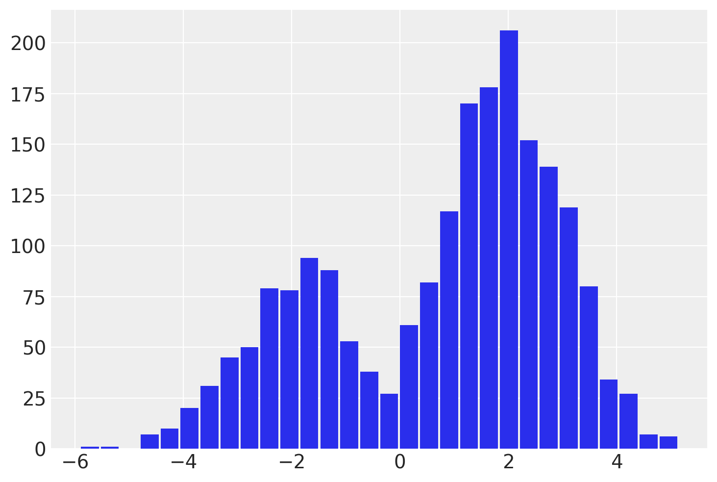
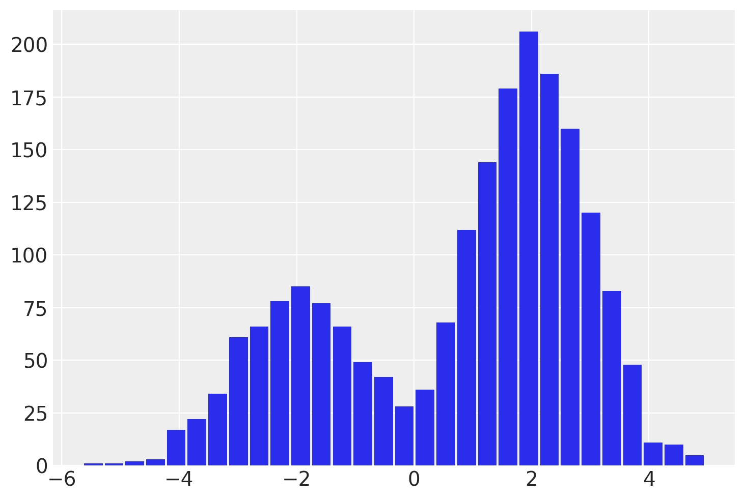
这个 idx 变量让我们在运行NUTS采样器后恢复混合分配变量！我们可以通过从每个样本的相关 idx 中读取混合标签来拆分 y 的样本。

# fmt: off
post = idata.posterior
plt.hist(
    post.where(post.idx == 0).y.values.reshape(-1),
    bins=30,
    rwidth=0.9,
    alpha=0.75,
    label='idx = 0',
)
plt.hist(
    post.where(post.idx == 1).y.values.reshape(-1),
    bins=30,
    rwidth=0.9,
    alpha=0.75,
    label='idx = 1'
)
# fmt: on
plt.legend();

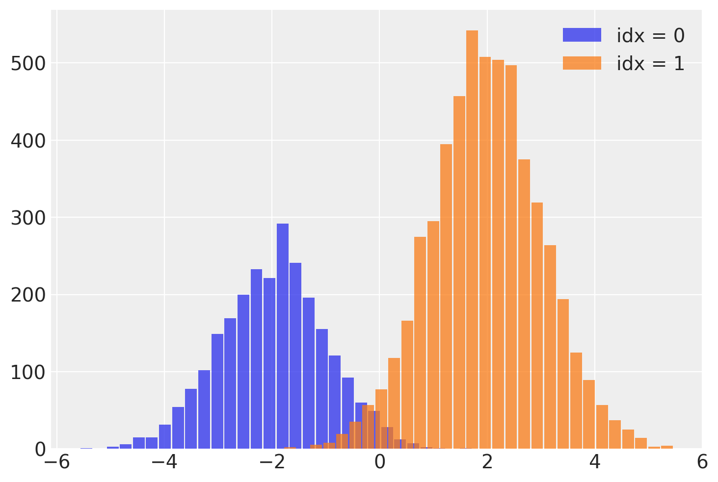
需要注意的一个重要问题是，这个离散变量的有效样本量（ESS）较低，特别是在尾部。这意味着idx可能无法很好地估计，特别是在尾部。如果这一点很重要，我建议使用lp_idx，它是给定每次迭代样本值的idx的对数概率。在下一个示例中将进一步探讨使用lp_idx的好处。

煤矿开采模型

同样的方法也适用于煤矿开采转折点模型。煤矿开采数据集记录了1851年至1962年间英国煤矿灾难的数量。该时间序列数据集捕捉到了正在引入采矿安全法规的时期，我们尝试使用一个离散的转折点变量来估计这一事件发生的时间。

# fmt: off
disaster_data = pd.Series(
    [4, 5, 4, 0, 1, 4, 3, 4, 0, 6, 3, 3, 4, 0, 2, 6,
    3, 3, 5, 4, 5, 3, 1, 4, 4, 1, 5, 5, 3, 4, 2, 5,
    2, 2, 3, 4, 2, 1, 3, np.nan, 2, 1, 1, 1, 1, 3, 0, 0,
    1, 0, 1, 1, 0, 0, 3, 1, 0, 3, 2, 2, 0, 1, 1, 1,
    0, 1, 0, 1, 0, 0, 0, 2, 1, 0, 0, 0, 1, 1, 0, 2,
    3, 3, 1, np.nan, 2, 1, 1, 1, 1, 2, 4, 2, 0, 0, 1, 4,
    0, 0, 0, 1, 0, 0, 0, 0, 0, 1, 0, 0, 1, 0, 1]
)

# fmt: on
years = np.arange(1851, 1962)

with pmx.MarginalModel() as disaster_model:
    switchpoint = pm.DiscreteUniform("switchpoint", lower=years.min(), upper=years.max())
    early_rate = pm.Exponential("early_rate", 1.0, initval=3)
    late_rate = pm.Exponential("late_rate", 1.0, initval=1)
    rate = pm.math.switch(switchpoint >= years, early_rate, late_rate)
    disasters = pm.Poisson("disasters", rate, observed=disaster_data)

/home/zv/upstream/pymc/pymc/model/core.py:1307: RuntimeWarning: invalid value encountered in cast
  data = convert_observed_data(data).astype(rv_var.dtype)
/home/zv/upstream/pymc/pymc/model/core.py:1321: ImputationWarning: Data in disasters contains missing values and will be automatically imputed from the sampling distribution.
  warnings.warn(impute_message, ImputationWarning)

我们将在边缘化switchpoint变量之前和之后对模型进行采样

with disaster_model:
    before_marg = pm.sample(chains=2, random_seed=rng)

disaster_model.marginalize(["switchpoint"])

with disaster_model:
    after_marg = pm.sample(chains=2, random_seed=rng)

Multiprocess sampling (2 chains in 2 jobs)
CompoundStep
>CompoundStep
>>Metropolis: [switchpoint]
>>Metropolis: [disasters_unobserved]
>NUTS: [early_rate, late_rate]

100.00% [4000/4000 00:07<00:00 Sampling 2 chains, 0 divergences]

Sampling 2 chains for 1_000 tune and 1_000 draw iterations (2_000 + 2_000 draws total) took 8 seconds.
We recommend running at least 4 chains for robust computation of convergence diagnostics
/home/zv/upstream/pymc-experimental/pymc_experimental/model/marginal_model.py:169: UserWarning: There are multiple dependent variables in a FiniteDiscreteMarginalRV. Their joint logp terms will be assigned to the first RV: disasters_unobserved
  warnings.warn(
Multiprocess sampling (2 chains in 2 jobs)
CompoundStep
>NUTS: [early_rate, late_rate]
>Metropolis: [disasters_unobserved]

100.00% [4000/4000 03:11<00:00 Sampling 2 chains, 0 divergences]

Sampling 2 chains for 1_000 tune and 1_000 draw iterations (2_000 + 2_000 draws total) took 191 seconds.
We recommend running at least 4 chains for robust computation of convergence diagnostics

az.summary(before_marg, var_names=["~disasters"], filter_vars="like")

	mean	sd	hdi_3%	hdi_97%	mcse_mean	mcse_sd	ess_bulk	ess_tail	r_hat
switchpoint	1890.224	2.657	1886.000	1896.000	0.192	0.136	201.0	171.0	1.0
early_rate	3.085	0.279	2.598	3.636	0.007	0.005	1493.0	1255.0	1.0
late_rate	0.927	0.114	0.715	1.143	0.003	0.002	1136.0	1317.0	1.0

az.summary(after_marg, var_names=["~disasters"], filter_vars="like")

	mean	sd	hdi_3%	hdi_97%	mcse_mean	mcse_sd	ess_bulk	ess_tail	r_hat
early_rate	3.077	0.289	2.529	3.606	0.007	0.005	1734.0	1150.0	1.0
late_rate	0.932	0.113	0.725	1.150	0.003	0.002	1871.0	1403.0	1.0

如前所述，ESS得到了极大的改善

最后，让我们恢复switchpoint变量

disaster_model.recover_marginals(after_marg);

az.summary(after_marg, var_names=["~disasters", "~lp"], filter_vars="like")

	mean	sd	hdi_3%	hdi_97%	mcse_mean	mcse_sd	ess_bulk	ess_tail	r_hat
early_rate	3.077	0.289	2.529	3.606	0.007	0.005	1734.0	1150.0	1.00
late_rate	0.932	0.113	0.725	1.150	0.003	0.002	1871.0	1403.0	1.00
switchpoint	1889.764	2.458	1886.000	1894.000	0.070	0.050	1190.0	1883.0	1.01

虽然 recover_marginals 能够对被边缘化的离散变量进行采样。每次抽样所关联的概率通常能提供一个更清晰的离散变量估计。特别是对于较低概率值的情况。通过比较采样值的直方图与对数概率图，可以最好地说明这一点。

post = after_marg.posterior.switchpoint.values.reshape(-1)
bins = np.arange(post.min(), post.max())
plt.hist(post, bins, rwidth=0.9);

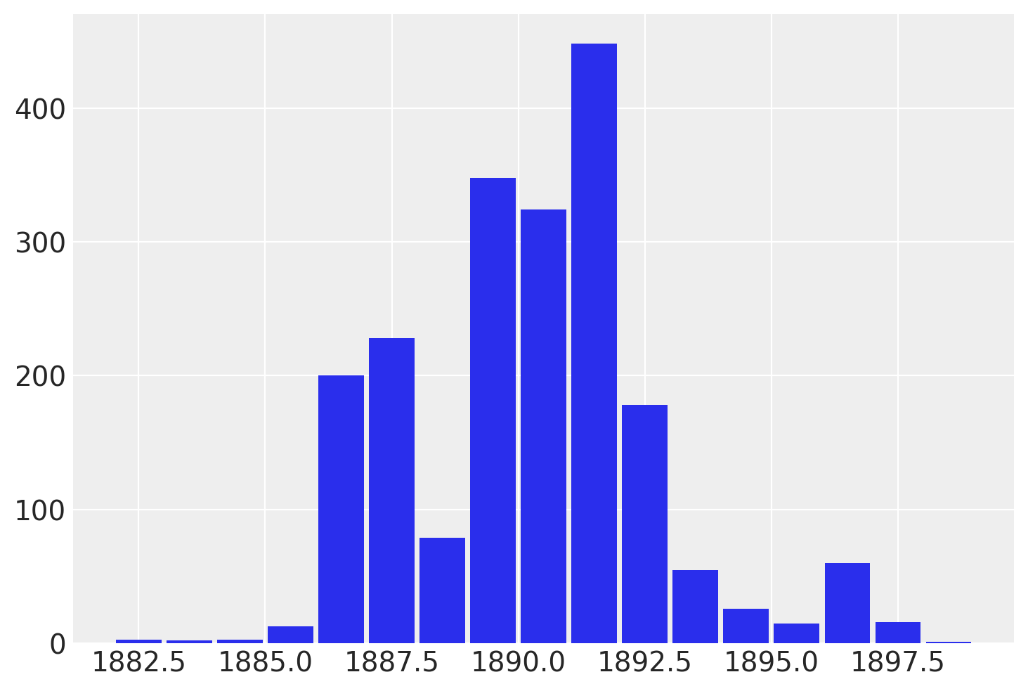
lp_switchpoint = after_marg.posterior.lp_switchpoint.mean(dim=["chain", "draw"])
x_max = years[lp_switchpoint.argmax()]

plt.scatter(years, lp_switchpoint)
plt.axvline(x=x_max, c="orange")
plt.xlabel(r"$\mathrm{year}$")
plt.ylabel(r"$\log p(\mathrm{switchpoint}=\mathrm{year})$");

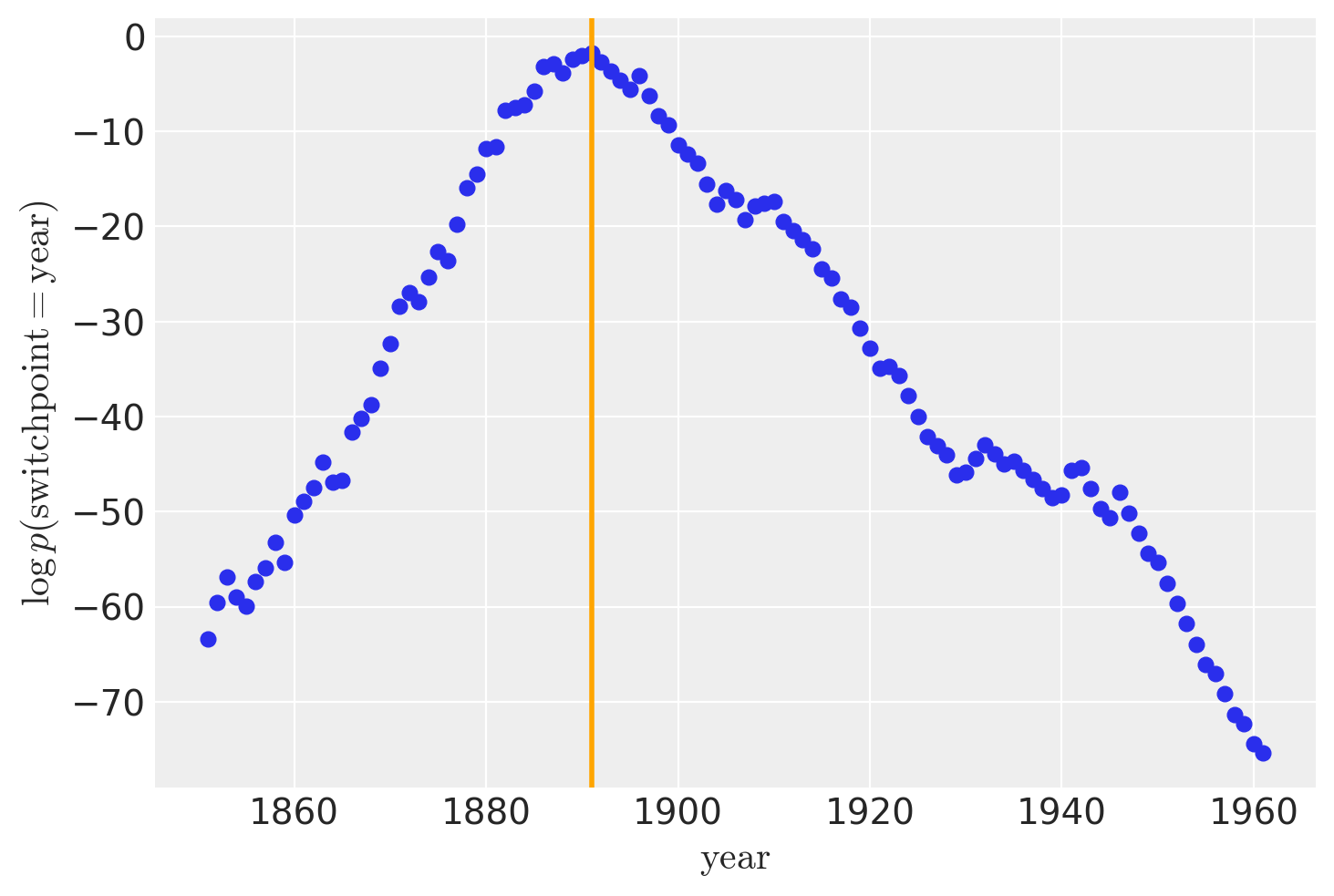
通过绘制采样值的直方图而不是直接处理对数概率，我们对底层离散分布的探索变得更加嘈杂和不完整。

作者

• 由Rob Zinkov于2024年1月撰写

参考资料

• STAN手册中关于边际化的章节

水印

%load_ext watermark
%watermark -n -u -v -iv -w -p pytensor,xarray

Last updated: Sat Feb 10 2024

Python implementation: CPython
Python version       : 3.11.6
IPython version      : 8.20.0

pytensor: 2.18.6
xarray  : 2023.11.0

pymc             : 5.11
numpy            : 1.26.3
pytensor         : 2.18.6
pymc_experimental: 0.0.15
arviz            : 0.17.0
pandas           : 2.1.4
matplotlib       : 3.8.2

Watermark: 2.4.3