


更新先验#
在本笔记本中,我们将展示在原理上,如何在新数据可用时更新先验。
注意事项
这个示例为我们展示了Interpolated类的一个非常好的使用示例。然而,在实践中这样做可能并不是一个好主意,不仅因为KDE被用来计算后验的pdf值,而且主要是因为用作先验的插值分布是一维的和不相关的。因此,即使它们在边缘上完美拟合,它们实际上并没有将我们从先前后验中获得的所有信息纳入模型中,特别是当后验变量相关时。关于这个主题的精彩讨论,请参阅Oriol Abril的博客文章Some dimensionality devils。
import arviz as az
import matplotlib as mpl
import matplotlib.pyplot as plt
import numpy as np
import pymc as pm
import pytensor.tensor as pt

from scipy import stats
from tqdm.notebook import trange

az.style.use("arviz-white")

%config InlineBackend.figure_format = "retina"
rng: np.random.Generator = np.random.default_rng(seed=42)
生成数据#
# True parameter values
alpha_true = 5
beta0_true = 7
beta1_true = 13
sigma_true = 2

# Size of dataset
size = 100

# Predictor variable
X1 = rng.normal(size=size)
X2 = rng.normal(size=size) * 0.2

# Simulate outcome variable
Y = alpha_true + beta0_true * X1 + beta1_true * X2 + rng.normal(size=size, scale=sigma_true)
模型规范#
我们对参数的初步信念相当有信息量(sigma=1),但与真实值有些偏差。
with pm.Model() as model:
    # Priors for unknown model parameters
    alpha = pm.Normal("alpha", mu=0, sigma=5)
    beta0 = pm.Normal("beta0", mu=0, sigma=5)
    beta1 = pm.Normal("beta1", mu=0, sigma=5)

    sigma = pm.HalfNormal("sigma", sigma=1)

    # Expected value of outcome
    mu = alpha + beta0 * X1 + beta1 * X2

    # Likelihood (sampling distribution) of observations
    Y_obs = pm.Normal("Y_obs", mu=mu, sigma=sigma, observed=Y)

    # draw 2_000 posterior samples
    trace = pm.sample(
        tune=1_500, draws=2_000, target_accept=0.9, progressbar=False, random_seed=rng
    )
Auto-assigning NUTS sampler...
Initializing NUTS using jitter+adapt_diag...
Multiprocess sampling (4 chains in 4 jobs)
NUTS: [alpha, beta0, beta1, sigma]
Sampling 4 chains for 1_500 tune and 2_000 draw iterations (6_000 + 8_000 draws total) took 2 seconds.
axes = az.plot_trace(
    data=trace,
    compact=True,
    lines=[
        ("alpha", {}, alpha_true),
        ("beta0", {}, beta0_true),
        ("beta1", {}, beta1_true),
        ("sigma", {}, sigma_true),
    ],
    backend_kwargs={"figsize": (12, 9), "layout": "constrained"},
)
plt.gcf().suptitle("Trace", fontsize=16);
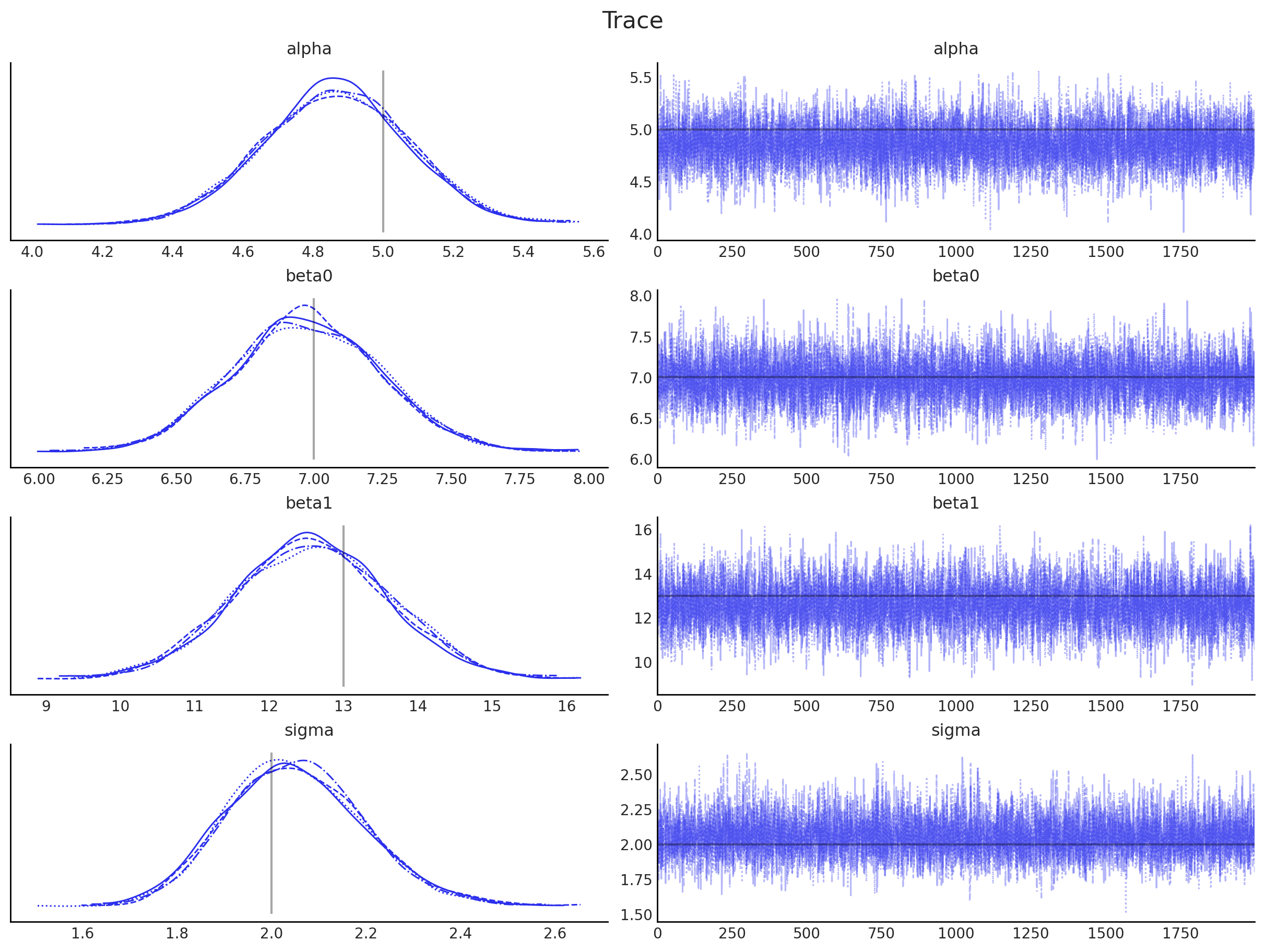
为了更新我们对参数的信念,我们使用后验分布,这些分布将作为下一次推理的先验分布。用于每次推理迭代的数据必须与前一次迭代的数据独立,否则相同的(可能是错误的)信念会一遍又一遍地注入系统中,放大错误并误导推理。通过确保数据是独立的,系统应该收敛到真实的参数值。
因为我们从后验分布中抽取样本(如上图右侧所示),我们需要估计它们的概率密度(如上图左侧所示)。核密度估计(KDE)是一种实现这一目标的方法,我们将在这里使用这种技术。无论如何,这是一个无法用解析式表达的经验分布。幸运的是,PyMC 提供了一种使用自定义分布的方法,通过 Interpolated 类。
def from_posterior(param, samples):
    smin, smax = samples.min().item(), samples.max().item()
    width = smax - smin
    x = np.linspace(smin, smax, 100)
    y = stats.gaussian_kde(samples)(x)

    # what was never sampled should have a small probability but not 0,
    # so we'll extend the domain and use linear approximation of density on it
    x = np.concatenate([[x[0] - 3 * width], x, [x[-1] + 3 * width]])
    y = np.concatenate([[0], y, [0]])
    return pm.Interpolated(param, x, y)
现在我们只需要生成更多数据并构建我们的贝叶斯模型,以便当前迭代的先验分布是前一次迭代的后验分布。仍然可以使用NUTS采样方法,因为Interpolated类实现了对哈密顿蒙特卡洛采样器所需的梯度计算。
traces = [trace]
n_iterations = 10

for _ in trange(n_iterations):
    # generate more data
    X1 = rng.normal(size=size)
    X2 = rng.normal(size=size) * 0.2
    Y = alpha_true + beta0_true * X1 + beta1_true * X2 + rng.normal(size=size, scale=sigma_true)

    with pm.Model() as model:
        # Priors are posteriors from previous iteration
        alpha = from_posterior("alpha", az.extract(trace, group="posterior", var_names=["alpha"]))
        beta0 = from_posterior("beta0", az.extract(trace, group="posterior", var_names=["beta0"]))
        beta1 = from_posterior("beta1", az.extract(trace, group="posterior", var_names=["beta1"]))
        sigma = from_posterior("sigma", az.extract(trace, group="posterior", var_names=["sigma"]))

        # Expected value of outcome
        mu = alpha + beta0 * X1 + beta1 * X2

        # Likelihood (sampling distribution) of observations
        Y_obs = pm.Normal("Y_obs", mu=mu, sigma=sigma, observed=Y)

        # draw 2_000 posterior samples
        trace = pm.sample(
            tune=1_500, draws=2_000, target_accept=0.9, progressbar=False, random_seed=rng
        )
        traces.append(trace)
Auto-assigning NUTS sampler...
Initializing NUTS using jitter+adapt_diag...
Multiprocess sampling (4 chains in 4 jobs)
NUTS: [alpha, beta0, beta1, sigma]
Sampling 4 chains for 1_500 tune and 2_000 draw iterations (6_000 + 8_000 draws total) took 2 seconds.
Auto-assigning NUTS sampler...
Initializing NUTS using jitter+adapt_diag...
Multiprocess sampling (4 chains in 4 jobs)
NUTS: [alpha, beta0, beta1, sigma]
Sampling 4 chains for 1_500 tune and 2_000 draw iterations (6_000 + 8_000 draws total) took 2 seconds.
Auto-assigning NUTS sampler...
Initializing NUTS using jitter+adapt_diag...
Multiprocess sampling (4 chains in 4 jobs)
NUTS: [alpha, beta0, beta1, sigma]
Sampling 4 chains for 1_500 tune and 2_000 draw iterations (6_000 + 8_000 draws total) took 2 seconds.
Auto-assigning NUTS sampler...
Initializing NUTS using jitter+adapt_diag...
Multiprocess sampling (4 chains in 4 jobs)
NUTS: [alpha, beta0, beta1, sigma]
Sampling 4 chains for 1_500 tune and 2_000 draw iterations (6_000 + 8_000 draws total) took 2 seconds.
Auto-assigning NUTS sampler...
Initializing NUTS using jitter+adapt_diag...
Multiprocess sampling (4 chains in 4 jobs)
NUTS: [alpha, beta0, beta1, sigma]
Sampling 4 chains for 1_500 tune and 2_000 draw iterations (6_000 + 8_000 draws total) took 2 seconds.
Auto-assigning NUTS sampler...
Initializing NUTS using jitter+adapt_diag...
Multiprocess sampling (4 chains in 4 jobs)
NUTS: [alpha, beta0, beta1, sigma]
Sampling 4 chains for 1_500 tune and 2_000 draw iterations (6_000 + 8_000 draws total) took 2 seconds.
Auto-assigning NUTS sampler...
Initializing NUTS using jitter+adapt_diag...
Multiprocess sampling (4 chains in 4 jobs)
NUTS: [alpha, beta0, beta1, sigma]
Sampling 4 chains for 1_500 tune and 2_000 draw iterations (6_000 + 8_000 draws total) took 4 seconds.
The rhat statistic is larger than 1.01 for some parameters. This indicates problems during sampling. See https://arxiv.org/abs/1903.08008 for details
The effective sample size per chain is smaller than 100 for some parameters.  A higher number is needed for reliable rhat and ess computation. See https://arxiv.org/abs/1903.08008 for details
Auto-assigning NUTS sampler...
Initializing NUTS using jitter+adapt_diag...
Multiprocess sampling (4 chains in 4 jobs)
NUTS: [alpha, beta0, beta1, sigma]
Sampling 4 chains for 1_500 tune and 2_000 draw iterations (6_000 + 8_000 draws total) took 3 seconds.
Auto-assigning NUTS sampler...
Initializing NUTS using jitter+adapt_diag...
Multiprocess sampling (4 chains in 4 jobs)
NUTS: [alpha, beta0, beta1, sigma]
Sampling 4 chains for 1_500 tune and 2_000 draw iterations (6_000 + 8_000 draws total) took 5 seconds.
The rhat statistic is larger than 1.01 for some parameters. This indicates problems during sampling. See https://arxiv.org/abs/1903.08008 for details
The effective sample size per chain is smaller than 100 for some parameters.  A higher number is needed for reliable rhat and ess computation. See https://arxiv.org/abs/1903.08008 for details
fig, ax = plt.subplots(nrows=4, ncols=1, figsize=(12, 12), sharex=False, sharey=False)

cmap = mpl.cm.viridis

for i, (param, true_value) in enumerate(
    zip(["alpha", "beta0", "beta1", "sigma"], [alpha_true, beta0_true, beta1_true, sigma_true])
):
    for update_i, trace in enumerate(traces):
        samples = az.extract(trace, group="posterior", var_names=param)
        smin, smax = np.min(samples), np.max(samples)
        x = np.linspace(smin, smax, 100)
        y = stats.gaussian_kde(samples)(x)
        ax[i].plot(x, y, color=cmap(1 - update_i / len(traces)))
        ax[i].axvline(true_value, c="k")
        ax[i].set(title=param)
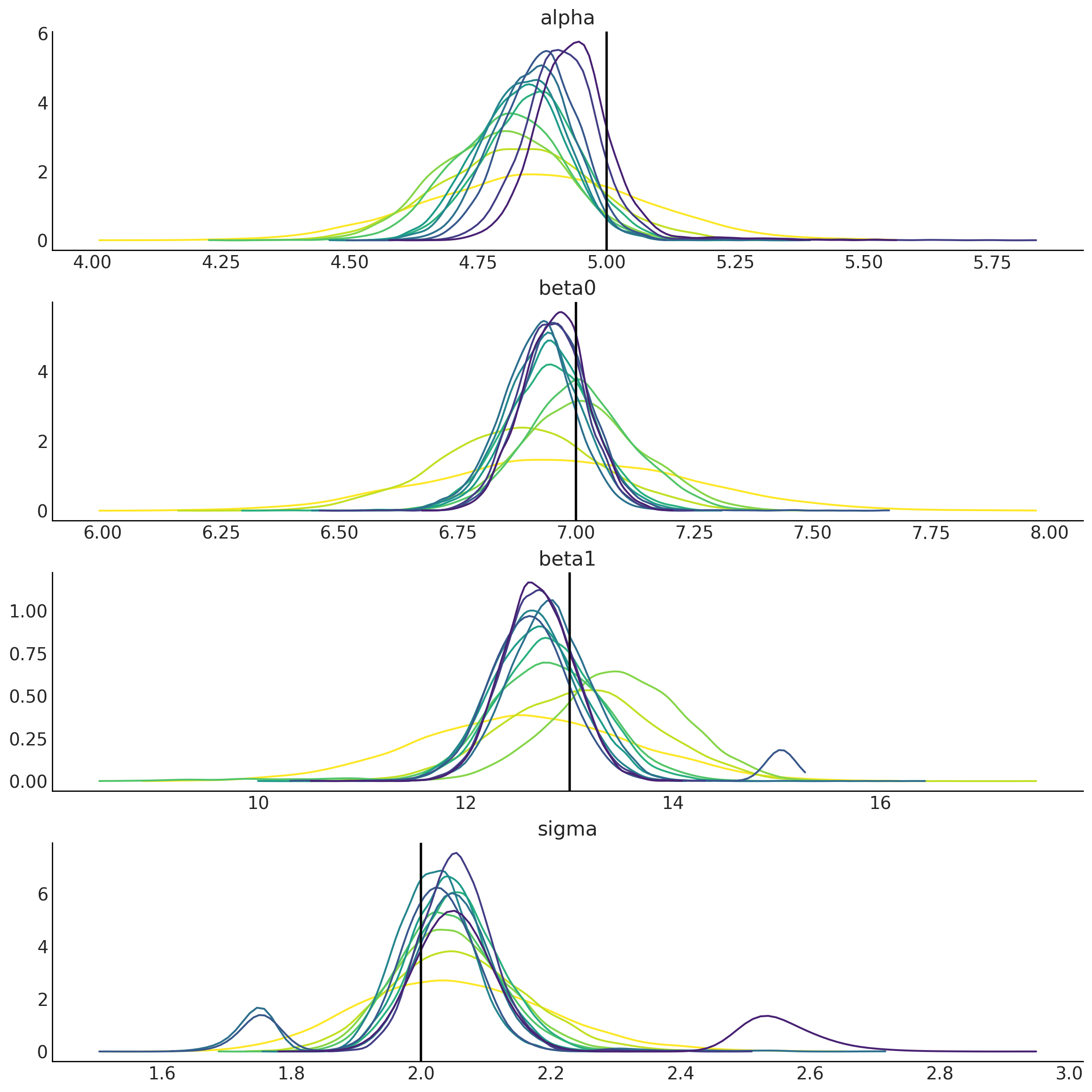
您可以重新执行最后两个单元格以生成更多更新。
值得注意的是,我们参数的后验分布往往集中在它们的真值(垂直线)上,并且分布变得越来越窄。这意味着我们每次都变得更加自信,而最初(错误)的信念被我们纳入的新数据冲刷掉了。
并非万能药
需要注意的是,尽管迭代似乎在改进,但其中一些并不那么好,甚至有时看起来会退步。除了笔记本开头提到的几个原因外,在过程中还有几个关键步骤涉及随机性。因此,平均而言,情况应该会有所改善。
新观测值是随机的。如果在初始迭代中我们得到的值接近分布的主体部分,然后我们连续得到几个来自正尾的值,那么在我们积累了几次来自尾部的抽取的迭代中,可能会出现偏差,并且“看起来比之前的更差”。
MCMC 是随机的。即使它收敛了,MCMC 也是一个随机过程,因此对
pymc.sample的不同调用将返回围绕精确后验分布的值,但并不总是相同的;我们可以预期多大的变化可以通过arviz.mcse()进行检查。KDE 也包含了这种通常可以忽略但确实存在的后验估计不确定性,生成的插值分布也是如此。
另一种方法
在 pymc-experimental 中,有一种替代方法是通过函数 prior_from_idata() 来实现类似的功能。这个函数:
使用MvNormal近似从后验创建先验。 该近似使用MvNormal分布。请记住,此函数仅适用于单峰后验,并且在复杂交互发生时将失败。此外,如果检索到的变量受到约束,您应为该变量指定一个变换,例如
log()用于标准差后验。