高斯混合模型

一个混合模型允许我们对数据分布的组成部分进行推断。更具体地说，高斯混合模型允许我们对指定数量的底层高斯分布的均值和标准差进行推断。

这可以在许多方面发挥作用。例如，我们可能对简单地以参数方式描述复杂分布感兴趣（即混合分布）。或者，我们可能对分类感兴趣，其中我们试图概率性地分类一个特定观察属于哪一类。

import arviz as az
import matplotlib.pyplot as plt
import numpy as np
import pandas as pd
import pymc as pm

from scipy.stats import norm
from xarray_einstats.stats import XrContinuousRV

%config InlineBackend.figure_format = 'retina'
RANDOM_SEED = 8927
rng = np.random.default_rng(RANDOM_SEED)
az.style.use("arviz-darkgrid")

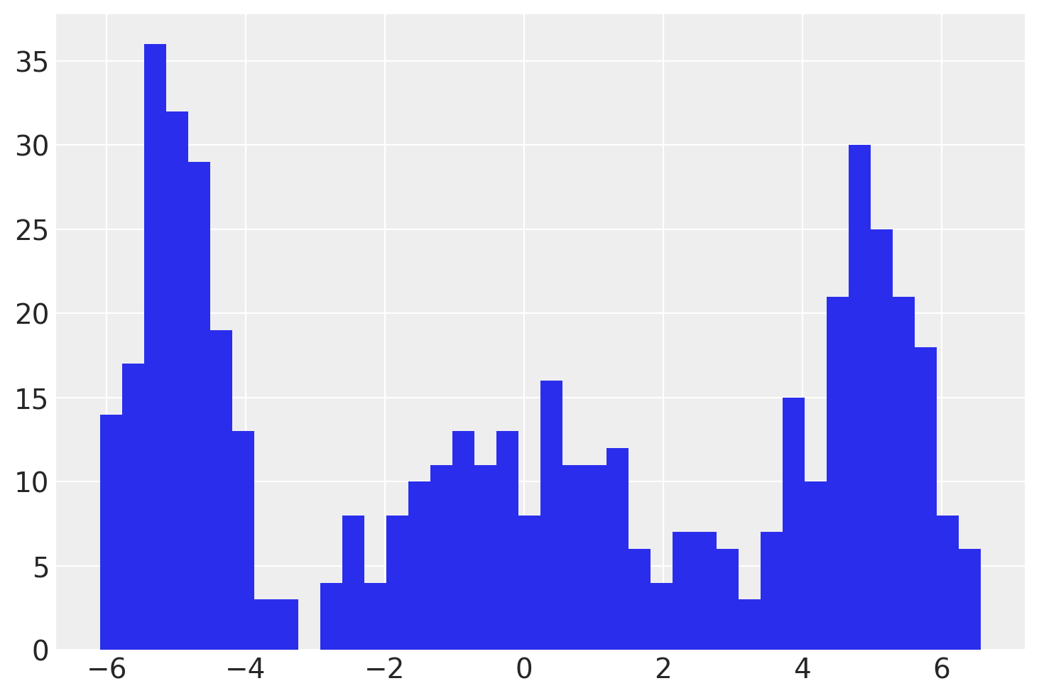
首先我们生成一些模拟的观测数据。

Show code cell source Hide code cell source

k = 3
ndata = 500
centers = np.array([-5, 0, 5])
sds = np.array([0.5, 2.0, 0.75])
idx = rng.integers(0, k, ndata)
x = rng.normal(loc=centers[idx], scale=sds[idx], size=ndata)
plt.hist(x, 40);

在PyMC模型中，我们将为每个3个聚类估计一个\(\mu\)和一个\(\sigma\)。使用pm.NormalMixture分布编写高斯混合模型非常容易。

with pm.Model(coords={"cluster": range(k)}) as model:
    μ = pm.Normal(
        "μ",
        mu=0,
        sigma=5,
        transform=pm.distributions.transforms.univariate_ordered,
        initval=[-4, 0, 4],
        dims="cluster",
    )
    σ = pm.HalfNormal("σ", sigma=1, dims="cluster")
    weights = pm.Dirichlet("w", np.ones(k), dims="cluster")
    pm.NormalMixture("x", w=weights, mu=μ, sigma=σ, observed=x)

pm.model_to_graphviz(model)

with model:
    idata = pm.sample()

Auto-assigning NUTS sampler...
Initializing NUTS using jitter+adapt_diag...
Multiprocess sampling (4 chains in 4 jobs)
NUTS: [μ, σ, w]

100.00% [8000/8000 00:03<00:00 Sampling 4 chains, 0 divergences]

Sampling 4 chains for 1_000 tune and 1_000 draw iterations (4_000 + 4_000 draws total) took 4 seconds.

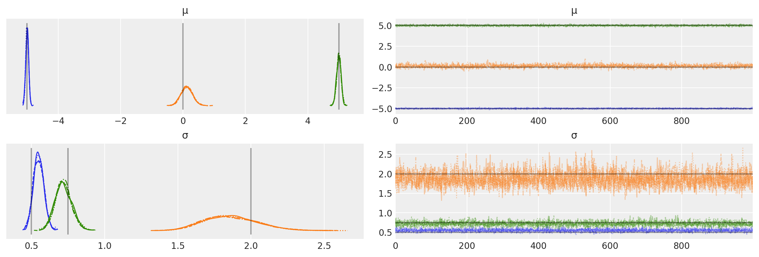
我们还可以绘制轨迹以检查MCMC链的性质，并与真实值进行比较。

az.plot_trace(idata, var_names=["μ", "σ"], lines=[("μ", {}, [centers]), ("σ", {}, [sds])]);

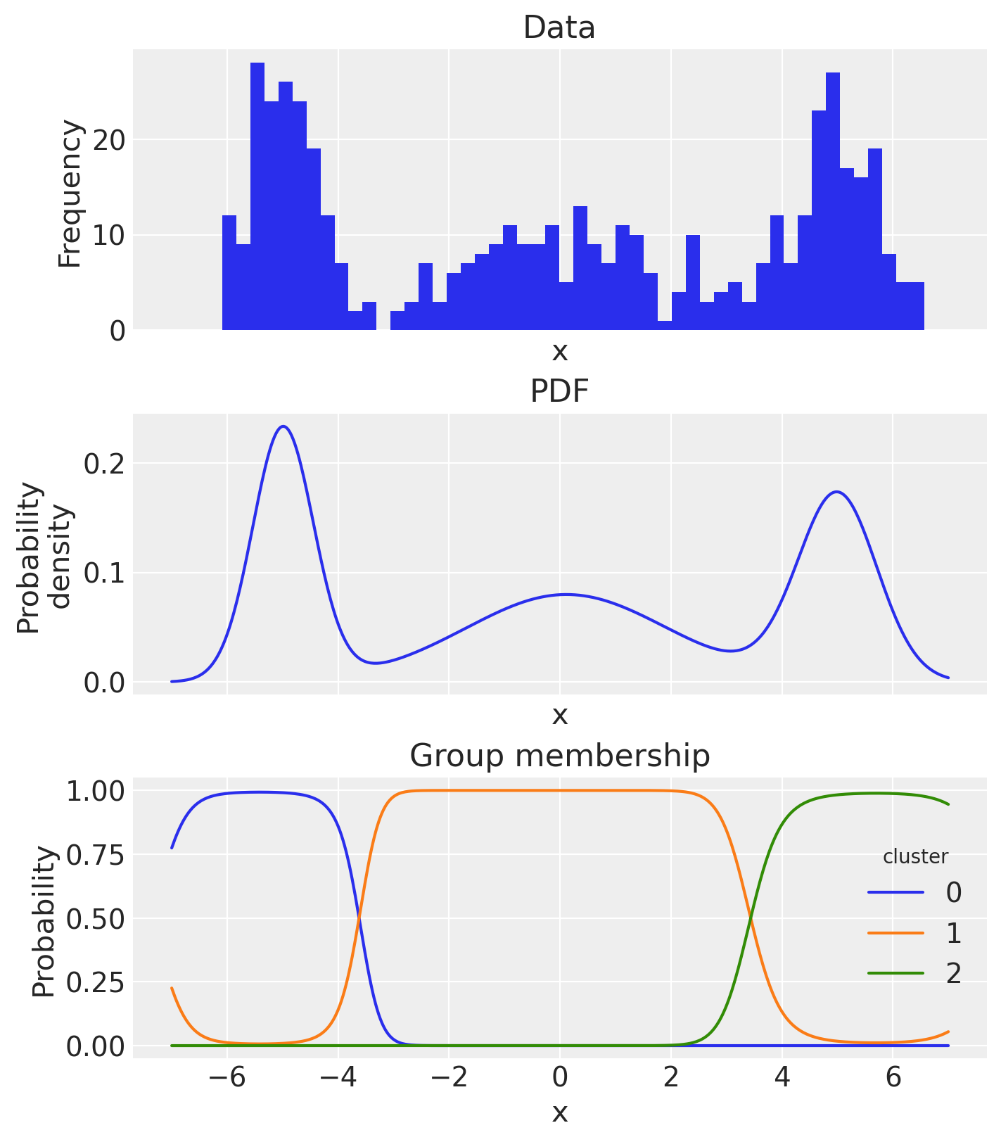
如果我们愿意，我们可以计算概率密度函数并检查基于后验均值估计的估计群体成员概率。

xi = np.linspace(-7, 7, 500)
post = idata.posterior
pdf_components = XrContinuousRV(norm, post["μ"], post["σ"]).pdf(xi) * post["w"]
pdf = pdf_components.sum("cluster")

fig, ax = plt.subplots(3, 1, figsize=(7, 8), sharex=True)
# empirical histogram
ax[0].hist(x, 50)
ax[0].set(title="Data", xlabel="x", ylabel="Frequency")
# pdf
pdf_components.mean(dim=["chain", "draw"]).sum("cluster").plot.line(ax=ax[1])
ax[1].set(title="PDF", xlabel="x", ylabel="Probability\ndensity")
# plot group membership probabilities
(pdf_components / pdf).mean(dim=["chain", "draw"]).plot.line(hue="cluster", ax=ax[2])
ax[2].set(title="Group membership", xlabel="x", ylabel="Probability");

作者

• 由Abe Flaxman撰写。

• 由Thomas Wiecki更新。

• 由 Benjamin T. Vincent 于2022年4月更新（#310）以使用 pm.NormalMixture。

• 由Benjamin T. Vincent于2023年2月更新，以在PyMC v5上运行。

水印

%load_ext watermark
%watermark -n -u -v -iv -w -p pytensor,aeppl,xarray,xarray_einstats

Last updated: Wed Feb 01 2023

Python implementation: CPython
Python version       : 3.11.0
IPython version      : 8.9.0

pytensor       : 2.8.11
aeppl          : not installed
xarray         : 2023.1.0
xarray_einstats: 0.5.1

pymc      : 5.0.1
arviz     : 0.14.0
numpy     : 1.24.1
pandas    : 1.5.3
matplotlib: 3.6.3

Watermark: 2.3.1