使用多种方法进行贝叶斯推断的ODE Lotka-Volterra#

import arviz as az
import matplotlib.pyplot as plt
import numpy as np
import pandas as pd
import pymc as pm
import pytensor
import pytensor.tensor as pt

from numba import njit
from pymc.ode import DifferentialEquation
from pytensor.compile.ops import as_op
from scipy.integrate import odeint
from scipy.optimize import least_squares

print(f"Running on PyMC v{pm.__version__}")

Running on PyMC v5.1.2+24.gf3ce16f26

%load_ext watermark
az.style.use("arviz-darkgrid")
rng = np.random.default_rng(1234)

目的#

本笔记本的目的是演示如何在具有和不具有梯度的情况下对常微分方程（ODE）系统进行贝叶斯推断。比较了不同采样器的准确性和效率。

我们将首先介绍Lotka-Volterra捕食者-猎物ODE模型和示例数据。接下来，我们将使用scipy.odeint和（非贝叶斯）最小二乘优化来求解ODE。然后，我们使用PyMC中的非基于梯度的采样器进行贝叶斯推断。最后，我们使用基于梯度的采样器并比较结果。

关键结论#

基于本笔记本中的实验，对Lotka-Volterra方程进行贝叶斯推断的最简单有效的方法是：在Scipy中指定ODE系统，将函数包装为Pytensor操作，并在PyMC中使用差分进化Metropolis（DEMetropolis）采样器。

背景#

动机#

常微分方程模型（ODEs）用于各种科学和工程领域，以模拟物理变量随时间的变化。在给定实验数据的情况下，估计模型参数的值和不确定性的自然选择是贝叶斯推断。然而，在贝叶斯框架中，ODEs可能难以指定和求解，因此，本笔记本通过多种方法使用PyMC解决ODE推断问题。本例中使用的Lotka-Volterra模型经常用于基准测试贝叶斯推断方法（例如，在此Stan 案例研究，以及《统计反思》第16章中 [McElreath, 2018]）。

Lotka-Volterra 捕食者-猎物模型#

Lotka-Volterra模型描述了捕食者和猎物种群之间的相互作用。这个由以下ODE给出：

\[\begin{split} \begin{aligned} \frac{d x}{dt} &=\alpha x -\beta xy \\ \frac{d y}{dt} &=-\gamma y + \delta xy \end{aligned} \end{split}\]

状态向量 \(X(t)=[x(t),y(t)]\) 分别表示猎物和捕食者的密度。参数 \(\boldsymbol{\theta}=[\alpha,\beta,\gamma,\delta, x(0),y(0)]\) 是我们希望从实验观察中推断的未知数。\(x(0), y(0)\) 是求解ODE所需的状态的初始值，而 \(\alpha,\beta,\gamma\) 和 \(\delta\) 是表示以下内容的未知模型参数：

\(\alpha\) 是没有捕食者时猎物的增长速率。
\(\beta\) 是由于捕食导致的猎物死亡率。
\(\gamma\) 是当没有猎物时捕食者的死亡率。
\(\delta\) 是捕食者在有猎物存在时的增长速率。

哈德逊湾公司数据#

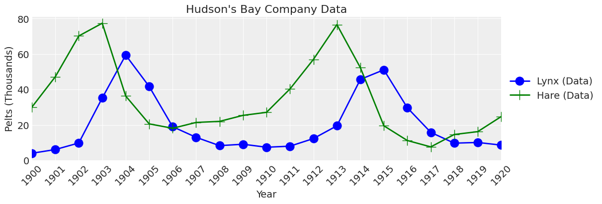
Lotka-Volterra捕食者-猎物模型已被成功用于解释捕食者和猎物自然种群的动态，例如哈德逊湾公司的猞猁和雪鞋兔数据。由于数据集较小，我们将手动输入这些值。

# fmt: off
data = pd.DataFrame(dict(
    year = np.arange(1900., 1921., 1),
    lynx = np.array([4.0, 6.1, 9.8, 35.2, 59.4, 41.7, 19.0, 13.0, 8.3, 9.1, 7.4,
                8.0, 12.3, 19.5, 45.7, 51.1, 29.7, 15.8, 9.7, 10.1, 8.6]),
    hare = np.array([30.0, 47.2, 70.2, 77.4, 36.3, 20.6, 18.1, 21.4, 22.0, 25.4, 
                 27.1, 40.3, 57.0, 76.6, 52.3, 19.5, 11.2, 7.6, 14.6, 16.2, 24.7])))
data.head()
# fmt: on

	year	lynx	hare
0	1900.0	4.0	30.0
1	1901.0	6.1	47.2
2	1902.0	9.8	70.2
3	1903.0	35.2	77.4
4	1904.0	59.4	36.3

# plot data function for reuse later
def plot_data(ax, lw=2, title="Hudson's Bay Company Data"):
    ax.plot(data.year, data.lynx, color="b", lw=lw, marker="o", markersize=12, label="Lynx (Data)")
    ax.plot(data.year, data.hare, color="g", lw=lw, marker="+", markersize=14, label="Hare (Data)")
    ax.legend(fontsize=14, loc="center left", bbox_to_anchor=(1, 0.5))
    ax.set_xlim([1900, 1920])
    ax.set_ylim(0)
    ax.set_xlabel("Year", fontsize=14)
    ax.set_ylabel("Pelts (Thousands)", fontsize=14)
    ax.set_xticks(data.year.astype(int))
    ax.set_xticklabels(ax.get_xticks(), rotation=45)
    ax.set_title(title, fontsize=16)
    return ax

_, ax = plt.subplots(figsize=(12, 4))
plot_data(ax);

../../../_images/07e77a972517df91ac84d870e9b2c42ca3c9f6f92420d84a4ef85ff0eb59d895.png

问题陈述#

本次分析的目的是在不确定性的基础上，估计1900年至1920年哈德逊湾公司数据的Lotka-Volterra模型参数。

Scipy `odeint`#

在这里，我们创建一个Python函数，该函数表示ODE方程的右侧，并具有odeint函数所需的调用签名。请注意，Scipy的solve_ivp也可以使用，但在速度测试中，较旧的odeint函数更快，因此在本笔记本中使用。

# define the right hand side of the ODE equations in the Scipy odeint signature
from numba import njit


@njit
def rhs(X, t, theta):
    # unpack parameters
    x, y = X
    alpha, beta, gamma, delta, xt0, yt0 = theta
    # equations
    dx_dt = alpha * x - beta * x * y
    dy_dt = -gamma * y + delta * x * y
    return [dx_dt, dy_dt]

为了了解模型的运行情况并确保方程式正确工作，让我们用合理的\(\theta\)值运行一次模型并绘制结果。

# plot model function
def plot_model(
    ax,
    x_y,
    time=np.arange(1900, 1921, 0.01),
    alpha=1,
    lw=3,
    title="Hudson's Bay Company Data and\nExample Model Run",
):
    ax.plot(time, x_y[:, 1], color="b", alpha=alpha, lw=lw, label="Lynx (Model)")
    ax.plot(time, x_y[:, 0], color="g", alpha=alpha, lw=lw, label="Hare (Model)")
    ax.legend(fontsize=14, loc="center left", bbox_to_anchor=(1, 0.5))
    ax.set_title(title, fontsize=16)
    return ax

# note theta = alpha, beta, gamma, delta, xt0, yt0
theta = np.array([0.52, 0.026, 0.84, 0.026, 34.0, 5.9])
time = np.arange(1900, 1921, 0.01)

# call Scipy's odeint function
x_y = odeint(func=rhs, y0=theta[-2:], t=time, args=(theta,))

# plot
_, ax = plt.subplots(figsize=(12, 4))
plot_data(ax, lw=0)
plot_model(ax, x_y);

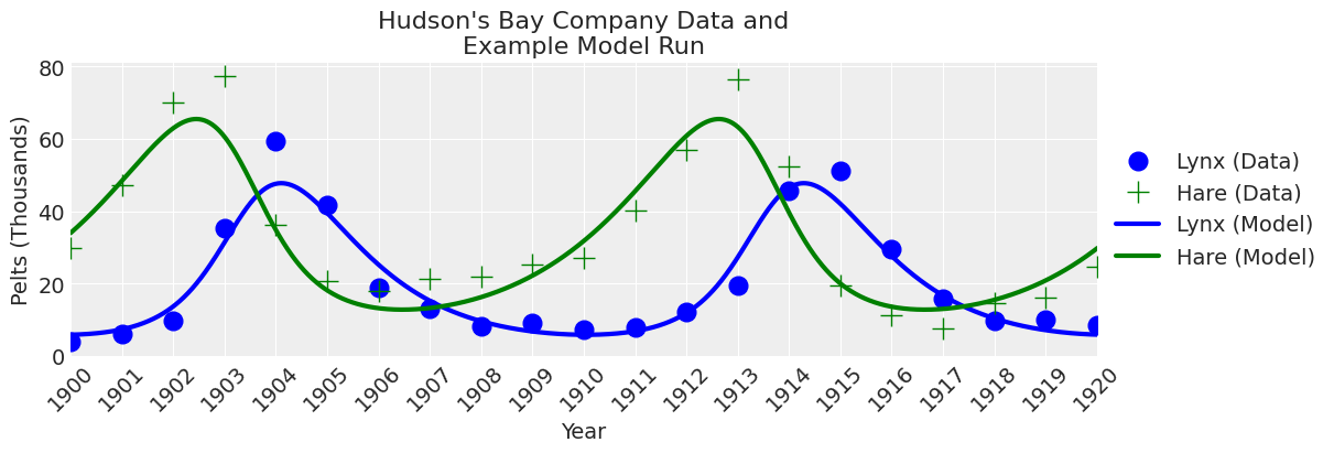
../../../_images/683533a99381191288ad88648de48554621102b799b09743d2eb44f39d509d4e.png

看起来odeint函数工作正常。

最小二乘解#

现在，我们可以使用最小二乘法来求解常微分方程。创建一个计算残差误差的函数。

# function that calculates residuals based on a given theta
def ode_model_resid(theta):
    return (
        data[["hare", "lynx"]] - odeint(func=rhs, y0=theta[-2:], t=data.year, args=(theta,))
    ).values.flatten()

将残差误差函数传递给 Scipy least_squares 求解器。

# calculate least squares using the Scipy solver
results = least_squares(ode_model_resid, x0=theta)

# put the results in a dataframe for presentation and convenience
df = pd.DataFrame()
parameter_names = ["alpha", "beta", "gamma", "delta", "h0", "l0"]
df["Parameter"] = parameter_names
df["Least Squares Solution"] = results.x
df.round(2)

	Parameter	Least Squares Solution
0	alpha	0.48
1	beta	0.02
2	gamma	0.93
3	delta	0.03
4	h0	34.91
5	l0	3.86

绘图

time = np.arange(1900, 1921, 0.01)
theta = results.x
x_y = odeint(func=rhs, y0=theta[-2:], t=time, args=(theta,))
fig, ax = plt.subplots(figsize=(12, 4))
plot_data(ax, lw=0)
plot_model(ax, x_y, title="Least Squares Solution");

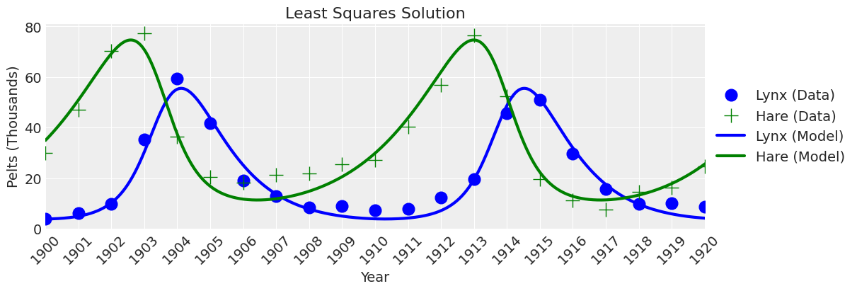
../../../_images/6d934292a361ea5776dc8a7042e67da6d40cbbdbc7044b26c403def31217638c.png

看起来没错。如果我们不关心不确定性，那么我们就完成了。但我们确实关心不确定性，所以让我们继续进行贝叶斯推断。

无梯度贝叶斯推断的PyMC模型规范#

与其他基于Numpy或Scipy的函数一样，scipy.integrate.odeint函数不能直接在PyMC模型中使用，因为PyMC需要知道变量的输入和输出类型才能进行编译。因此，我们使用一个Pytensor包装器来向PyMC提供变量类型。然后，该函数可以与无梯度采样器一起在PyMC中使用。

使用 @as_op 装饰器将 Python 函数转换为 Pytensor 操作符#

我们使用 @as_op 装饰器告诉 PyMC 输入变量类型和输出变量类型。 odeint 返回 Numpy 数组，但为此我们告诉 PyMC 它们是 Pytensor 双精度浮点张量。

# decorator with input and output types a Pytensor double float tensors
@as_op(itypes=[pt.dvector], otypes=[pt.dmatrix])
def pytensor_forward_model_matrix(theta):
    return odeint(func=rhs, y0=theta[-2:], t=data.year, args=(theta,))

PyMC 模型#

现在，我们可以使用微分方程求解器来指定 PyMC 模型！对于先验，我们将使用最小二乘计算的结果（results.x）来分配处于正确范围内的先验。这些是经验上得出的弱信息先验。我们还使它们在这个问题中仅取正值。

我们将使用未转换数据（即未进行对数转换）的正态似然来最好地拟合数据的峰值。

theta = results.x  # least squares solution used to inform the priors
with pm.Model() as model:
    # Priors
    alpha = pm.TruncatedNormal("alpha", mu=theta[0], sigma=0.1, lower=0, initval=theta[0])
    beta = pm.TruncatedNormal("beta", mu=theta[1], sigma=0.01, lower=0, initval=theta[1])
    gamma = pm.TruncatedNormal("gamma", mu=theta[2], sigma=0.1, lower=0, initval=theta[2])
    delta = pm.TruncatedNormal("delta", mu=theta[3], sigma=0.01, lower=0, initval=theta[3])
    xt0 = pm.TruncatedNormal("xto", mu=theta[4], sigma=1, lower=0, initval=theta[4])
    yt0 = pm.TruncatedNormal("yto", mu=theta[5], sigma=1, lower=0, initval=theta[5])
    sigma = pm.HalfNormal("sigma", 10)

    # Ode solution function
    ode_solution = pytensor_forward_model_matrix(
        pm.math.stack([alpha, beta, gamma, delta, xt0, yt0])
    )

    # Likelihood
    pm.Normal("Y_obs", mu=ode_solution, sigma=sigma, observed=data[["hare", "lynx"]].values)

pm.model_to_graphviz(model=model)

../../../_images/71f395975a2b788047b802bc081fe8dfd7c0427b4612a7d8fb24ba48d666934c.svg

绘图函数#

下面我们将重复使用几个绘图函数。

def plot_model_trace(ax, trace_df, row_idx, lw=1, alpha=0.2):
    cols = ["alpha", "beta", "gamma", "delta", "xto", "yto"]
    row = trace_df.iloc[row_idx, :][cols].values

    # alpha, beta, gamma, delta, Xt0, Yt0
    time = np.arange(1900, 1921, 0.01)
    theta = row
    x_y = odeint(func=rhs, y0=theta[-2:], t=time, args=(theta,))
    plot_model(ax, x_y, time=time, lw=lw, alpha=alpha);

def plot_inference(
    ax,
    trace,
    num_samples=25,
    title="Hudson's Bay Company Data and\nInference Model Runs",
    plot_model_kwargs=dict(lw=1, alpha=0.2),
):
    trace_df = az.extract(trace, num_samples=num_samples).to_dataframe()
    plot_data(ax, lw=0)
    for row_idx in range(num_samples):
        plot_model_trace(ax, trace_df, row_idx, **plot_model_kwargs)
    handles, labels = ax.get_legend_handles_labels()
    ax.legend(handles[:2], labels[:2], loc="center left", bbox_to_anchor=(1, 0.5))
    ax.set_title(title, fontsize=16)

无梯度采样器选项#

拥有良好的无梯度采样器可以扩展在PyMC中可以拟合的模型。在PyMC中，有五种适用于此问题的无梯度采样器选项：

Slice - 默认的无梯度采样器
DEMetropolisZ - 一种差分进化Metropolis采样器，使用过去的信息来指导采样跳跃
DEMetropolis - 一个差分进化Metropolis采样器
Metropolis - 普通的Metropolis采样器
SMC - 顺序蒙特卡罗

让我们试试看。

关于运行这些推理的一些注意事项。对于每个采样器，调整步数和抽取次数已减少，以在合理的时间内（大约几分钟）运行推理。在某些情况下，这不足以获得良好的推理结果，但足以用于演示目的。此外，在所有机器上，Pytensor op函数的多核处理无法正常工作，因此推理是在单个核心上执行的。

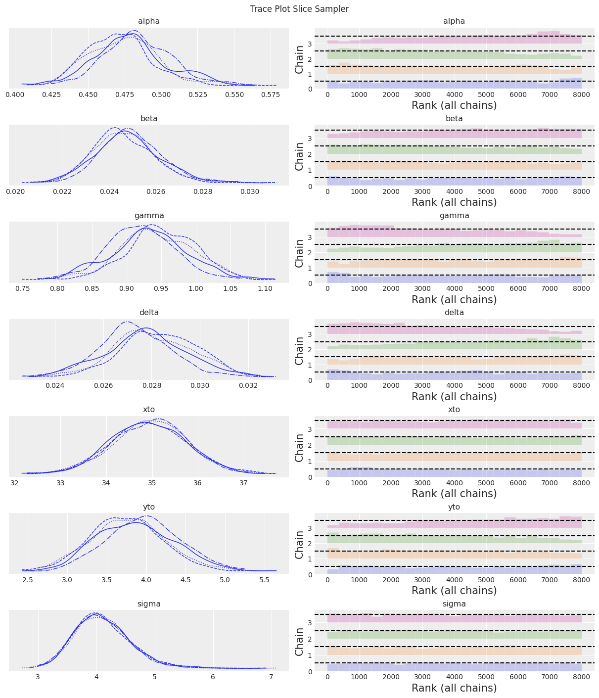
切片采样器#

# Variable list to give to the sample step parameter
vars_list = list(model.values_to_rvs.keys())[:-1]

# Specify the sampler
sampler = "Slice Sampler"
tune = draws = 2000

# Inference!
with model:
    trace_slice = pm.sample(step=[pm.Slice(vars_list)], tune=tune, draws=draws)
trace = trace_slice
az.summary(trace)

Multiprocess sampling (4 chains in 4 jobs)
CompoundStep
>Slice: [alpha]
>Slice: [beta]
>Slice: [gamma]
>Slice: [delta]
>Slice: [xto]
>Slice: [yto]
>Slice: [sigma]

100.00% [16000/16000 02:00<00:00 Sampling 4 chains, 0 divergences]

Sampling 4 chains for 2_000 tune and 2_000 draw iterations (8_000 + 8_000 draws total) took 120 seconds.
The rhat statistic is larger than 1.01 for some parameters. This indicates problems during sampling. See https://arxiv.org/abs/1903.08008 for details
The effective sample size per chain is smaller than 100 for some parameters.  A higher number is needed for reliable rhat and ess computation. See https://arxiv.org/abs/1903.08008 for details

	mean	sd	hdi_3%	hdi_97%	mcse_mean	mcse_sd	ess_bulk	ess_tail	r_hat
alpha	0.478	0.025	0.433	0.526	0.002	0.002	115.0	254.0	1.04
beta	0.025	0.001	0.022	0.027	0.000	0.000	253.0	497.0	1.01
gamma	0.937	0.054	0.835	1.039	0.005	0.004	109.0	241.0	1.04
delta	0.028	0.002	0.025	0.031	0.000	0.000	109.0	242.0	1.05
xto	34.945	0.823	33.386	36.472	0.023	0.016	1269.0	2646.0	1.00
yto	3.837	0.476	2.958	4.730	0.036	0.026	169.0	491.0	1.03
sigma	4.111	0.487	3.263	5.038	0.007	0.005	5141.0	5579.0	1.00

az.plot_trace(trace, kind="rank_bars")
plt.suptitle(f"Trace Plot {sampler}");

../../../_images/df4738e78f9859c808d3113aff088ad28256b6385f67b0683f975c70641a5a99.png

fig, ax = plt.subplots(figsize=(12, 4))
plot_inference(ax, trace, title=f"Data and Inference Model Runs\n{sampler} Sampler");

../../../_images/10e123cc546e62bac6f56148812be478c46c88943adc5a31dd5e7b32aabaed04.png

注释：
Slice 采样器速度较慢，导致有效样本量较低。尽管如此，结果开始看起来合理了！

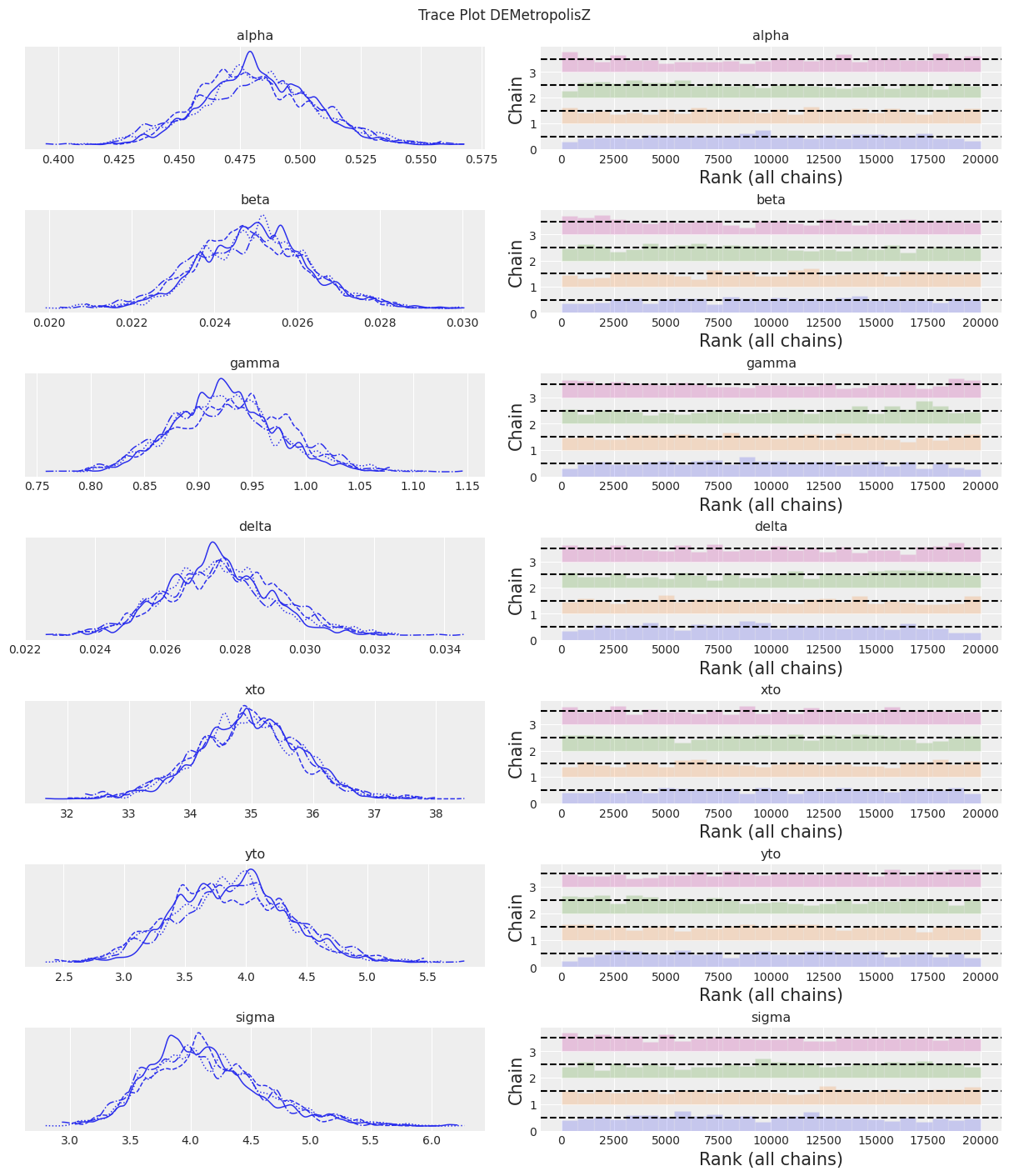
DE MetropolisZ 采样器#

sampler = "DEMetropolisZ"
tune = draws = 5000
with model:
    trace_DEMZ = pm.sample(step=[pm.DEMetropolisZ(vars_list)], tune=tune, draws=draws)
trace = trace_DEMZ
az.summary(trace)

Multiprocess sampling (4 chains in 4 jobs)
DEMetropolisZ: [alpha, beta, gamma, delta, xto, yto, sigma]

100.00% [40000/40000 00:16<00:00 Sampling 4 chains, 0 divergences]

Sampling 4 chains for 5_000 tune and 5_000 draw iterations (20_000 + 20_000 draws total) took 17 seconds.

	mean	sd	hdi_3%	hdi_97%	mcse_mean	mcse_sd	ess_bulk	ess_tail	r_hat
alpha	0.482	0.024	0.434	0.523	0.001	0.001	747.0	1341.0	1.01
beta	0.025	0.001	0.022	0.028	0.000	0.000	821.0	1415.0	1.00
gamma	0.927	0.051	0.834	1.023	0.002	0.001	896.0	1547.0	1.01
delta	0.028	0.002	0.025	0.031	0.000	0.000	783.0	1432.0	1.01
xto	34.938	0.847	33.314	36.479	0.029	0.021	855.0	1201.0	1.00
yto	3.887	0.473	2.983	4.724	0.017	0.012	777.0	1156.0	1.01
sigma	4.129	0.477	3.266	5.029	0.017	0.012	799.0	1466.0	1.00

az.plot_trace(trace, kind="rank_bars")
plt.suptitle(f"Trace Plot {sampler}");

../../../_images/5fa918d76b3e35d02809767abe1a63c7e2679bd4ab1d60069eb22763faf1ba70.png

fig, ax = plt.subplots(figsize=(12, 4))
plot_inference(ax, trace, title=f"Data and Inference\n{sampler} Sampler")

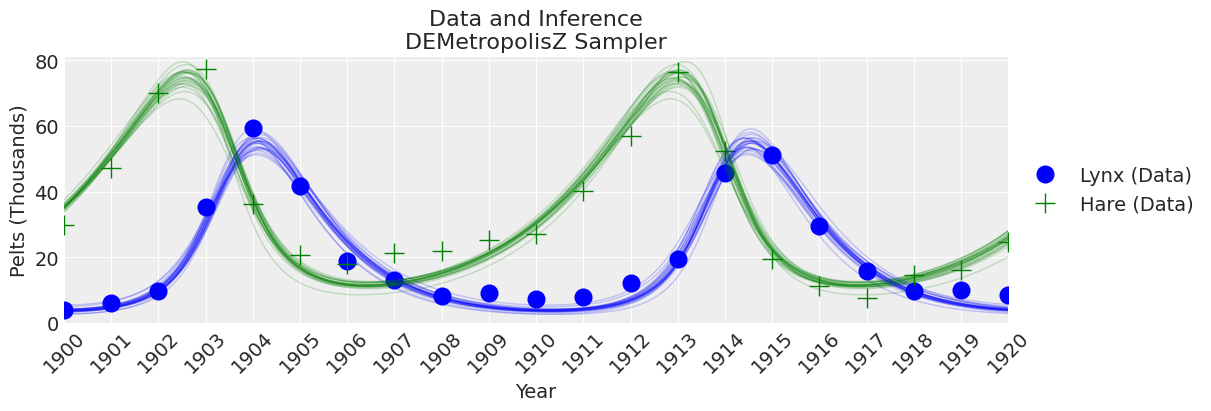
../../../_images/8c8aff02cfffa67c4a3a3ac3b6fbc4bece7462ce1eb9346beefe865f6be1df86.png

注释：
DEMetropolisZ 比 Slice 采样器更快地进行采样，因此在每分钟采样时间内具有更高的 ESS。参数估计值相似。“最终”推断仍需增加样本数量。

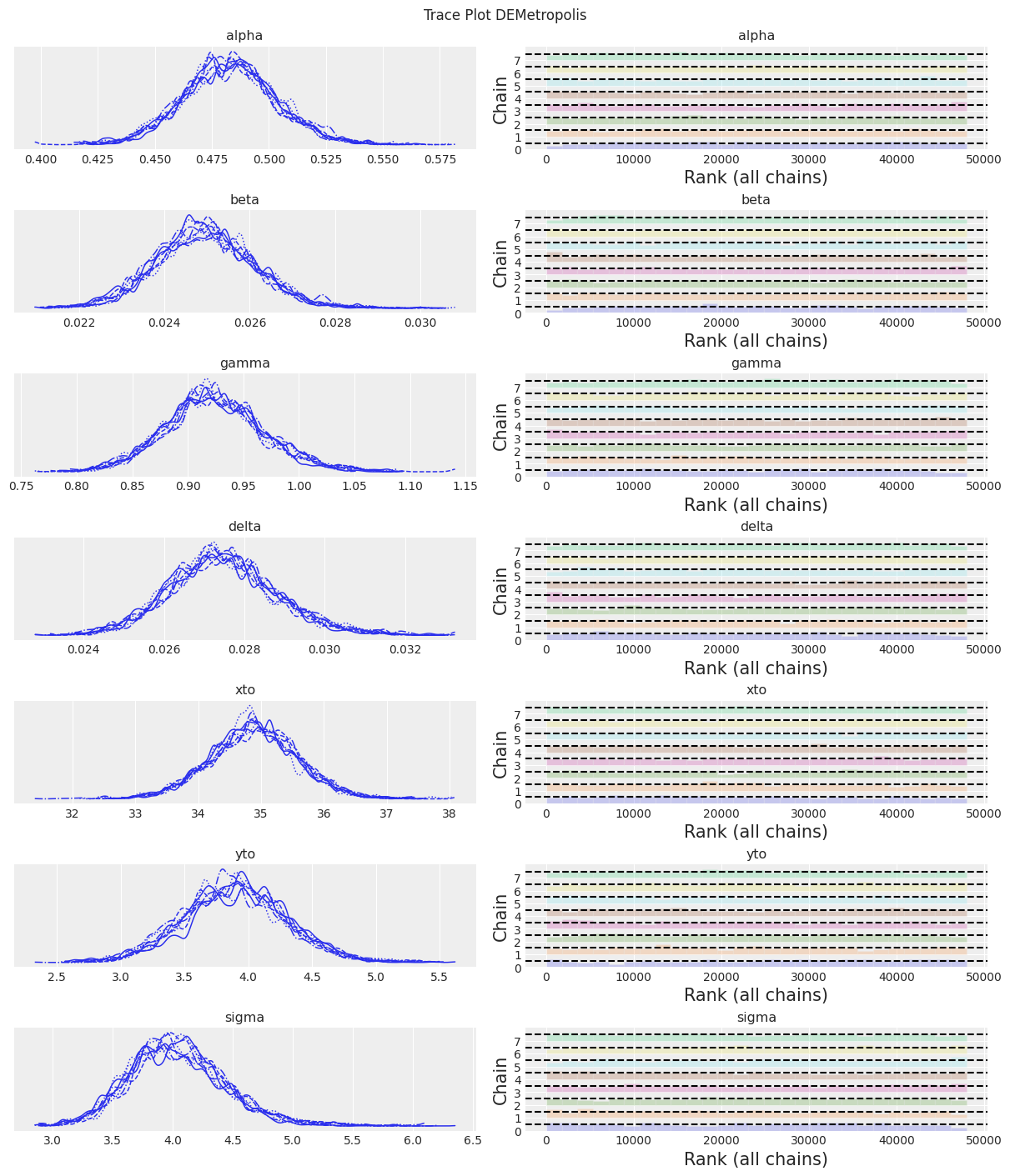
DEMetropolis 采样器#

在这些实验中，DEMetropolis 采样器不接受 tune 并且要求 chains 至少为 8。我们将抽取次数设置为 5000，像 3000 这样的较小数字会导致混合效果不佳。

sampler = "DEMetropolis"
chains = 8
draws = 6000
with model:
    trace_DEM = pm.sample(step=[pm.DEMetropolis(vars_list)], draws=draws, chains=chains)
trace = trace_DEM
az.summary(trace)

Population sampling (8 chains)
DEMetropolis: [alpha, beta, gamma, delta, xto, yto, sigma]
Attempting to parallelize chains to all cores. You can turn this off with `pm.sample(cores=1)`.

100.00% [8/8 00:00<00:00]

100.00% [7000/7000 00:39<00:00]

Sampling 8 chains for 1_000 tune and 6_000 draw iterations (8_000 + 48_000 draws total) took 40 seconds.

	mean	sd	hdi_3%	hdi_97%	mcse_mean	mcse_sd	ess_bulk	ess_tail	r_hat
alpha	0.483	0.021	0.443	0.520	0.000	0.000	1820.0	2647.0	1.00
beta	0.025	0.001	0.023	0.027	0.000	0.000	1891.0	3225.0	1.00
gamma	0.924	0.045	0.837	1.008	0.001	0.001	1818.0	2877.0	1.00
delta	0.027	0.001	0.025	0.030	0.000	0.000	1628.0	2469.0	1.00
xto	34.890	0.707	33.523	36.176	0.018	0.013	1484.0	2862.0	1.01
yto	3.897	0.403	3.126	4.644	0.010	0.007	1756.0	2468.0	1.00
sigma	4.042	0.405	3.335	4.836	0.011	0.008	1437.0	2902.0	1.00

az.plot_trace(trace, kind="rank_bars")
plt.suptitle(f"Trace Plot {sampler}");

../../../_images/0d16966368999982793a95c4ebbc079942cb841d7247f65cbac43c7c653a7b77.png

fig, ax = plt.subplots(figsize=(12, 4))
plot_inference(ax, trace, title=f"Data and Inference Model Runs\n{sampler} Sampler");

../../../_images/87c53756f4905c1c3b7e6c88438001abe7cffe73e95c9f7146d0ec0c57d9f37e.png

注释：
KDEs看起来过于波动，但ESS较高，R-hat值良好，rank_plots也看起来不错

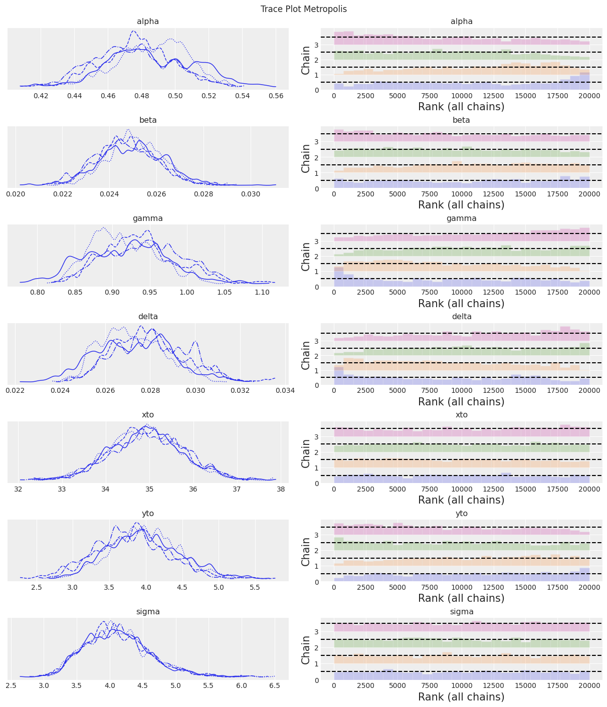
Metropolis Sampler#

sampler = "Metropolis"
tune = draws = 5000
with model:
    trace_M = pm.sample(step=[pm.Metropolis(vars_list)], tune=tune, draws=draws)
trace = trace_M
az.summary(trace)

Multiprocess sampling (4 chains in 4 jobs)
CompoundStep
>Metropolis: [alpha]
>Metropolis: [beta]
>Metropolis: [gamma]
>Metropolis: [delta]
>Metropolis: [xto]
>Metropolis: [yto]
>Metropolis: [sigma]

100.00% [40000/40000 01:46<00:00 Sampling 4 chains, 0 divergences]

/home/osvaldo/anaconda3/envs/pymc/lib/python3.10/site-packages/scipy/integrate/_odepack_py.py:248: ODEintWarning: Excess work done on this call (perhaps wrong Dfun type). Run with full_output = 1 to get quantitative information.
  warnings.warn(warning_msg, ODEintWarning)
/home/osvaldo/anaconda3/envs/pymc/lib/python3.10/site-packages/scipy/integrate/_odepack_py.py:248: ODEintWarning: Excess work done on this call (perhaps wrong Dfun type). Run with full_output = 1 to get quantitative information.
  warnings.warn(warning_msg, ODEintWarning)
Sampling 4 chains for 5_000 tune and 5_000 draw iterations (20_000 + 20_000 draws total) took 106 seconds.
The rhat statistic is larger than 1.01 for some parameters. This indicates problems during sampling. See https://arxiv.org/abs/1903.08008 for details
The effective sample size per chain is smaller than 100 for some parameters.  A higher number is needed for reliable rhat and ess computation. See https://arxiv.org/abs/1903.08008 for details

	mean	sd	hdi_3%	hdi_97%	mcse_mean	mcse_sd	ess_bulk	ess_tail	r_hat
alpha	0.481	0.024	0.437	0.523	0.004	0.003	44.0	112.0	1.10
beta	0.025	0.001	0.023	0.027	0.000	0.000	123.0	569.0	1.05
gamma	0.928	0.052	0.836	1.022	0.008	0.005	44.0	93.0	1.10
delta	0.028	0.002	0.025	0.031	0.000	0.000	47.0	113.0	1.09
xto	34.928	0.833	33.396	36.513	0.029	0.021	808.0	1128.0	1.00
yto	3.892	0.492	3.026	4.878	0.055	0.039	81.0	307.0	1.04
sigma	4.116	0.496	3.272	5.076	0.009	0.007	2870.0	3372.0	1.00

az.plot_trace(trace, kind="rank_bars")
plt.suptitle(f"Trace Plot {sampler}");

../../../_images/daf529f1f132ed1f19cf22b99c40d00f5e5c934afa6e8f2f0fd927cab70b18d6.png

fig, ax = plt.subplots(figsize=(12, 4))
plot_inference(ax, trace, title=f"Data and Inference Model Runs\n{sampler} Sampler");

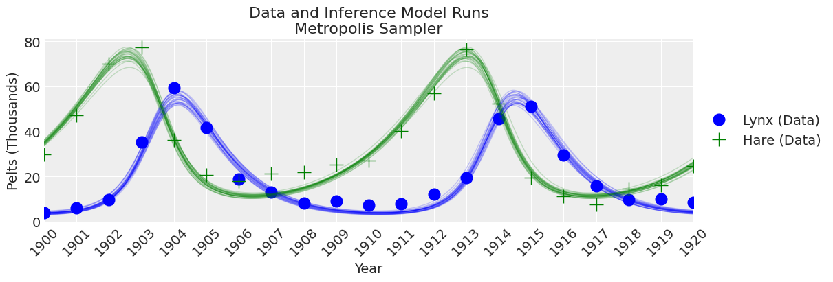
../../../_images/e68e06c8ab5de464507150ac16d69b47b64482f3376696b9372f7b5b80029aba.png

注意：
传统的Metropolis采样器比DEMetropolis采样器更不可靠且速度更慢。不推荐使用。

SMC采样器#

顺序蒙特卡罗（SMC）采样器可用于对常规贝叶斯模型进行采样，或在没有似然函数的情况下运行模型（近似贝叶斯计算）。让我们首先尝试一个常规模型，

带有似然函数的SMC#

sampler = "SMC with Likelihood"
draws = 2000
with model:
    trace_SMC_like = pm.sample_smc(draws)
trace = trace_SMC_like
az.summary(trace)

Initializing SMC sampler...
Sampling 4 chains in 4 jobs

100.00% [100/100 00:00<? Stage: 7 Beta: 1.000]

	mean	sd	hdi_3%	hdi_97%	mcse_mean	mcse_sd	ess_bulk	ess_tail	r_hat
alpha	0.482	0.025	0.436	0.527	0.000	0.000	8093.0	7636.0	1.0
beta	0.025	0.001	0.022	0.027	0.000	0.000	8090.0	7582.0	1.0
gamma	0.927	0.053	0.826	1.023	0.001	0.000	8064.0	8142.0	1.0
delta	0.028	0.002	0.025	0.031	0.000	0.000	8028.0	8016.0	1.0
xto	34.893	0.843	33.324	36.500	0.009	0.007	8060.0	7716.0	1.0
yto	3.889	0.480	2.997	4.796	0.005	0.004	7773.0	7884.0	1.0
sigma	4.123	0.497	3.243	5.057	0.006	0.004	8169.0	7971.0	1.0

trace.sample_stats._t_sampling

64.09551501274109

az.plot_trace(trace, kind="rank_bars")
plt.suptitle(f"Trace Plot {sampler}");

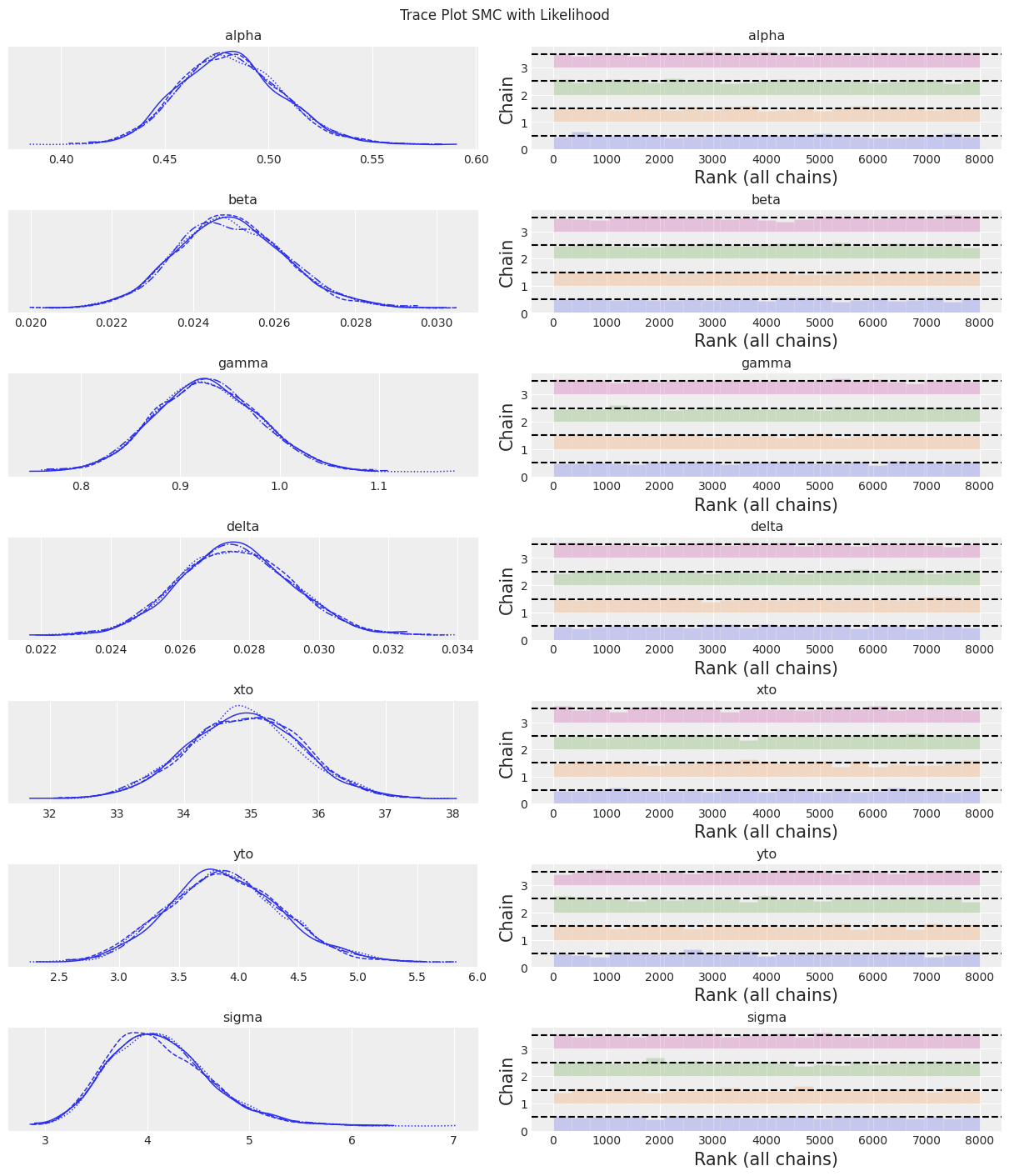
../../../_images/e860c173d9ce22cc8dfb8ba149a4f7192e4014e71bcc98a4ec1e729050532476.png

fig, ax = plt.subplots(figsize=(12, 4))
plot_inference(ax, trace, title=f"Data and Inference Model Runs\n{sampler} Sampler");

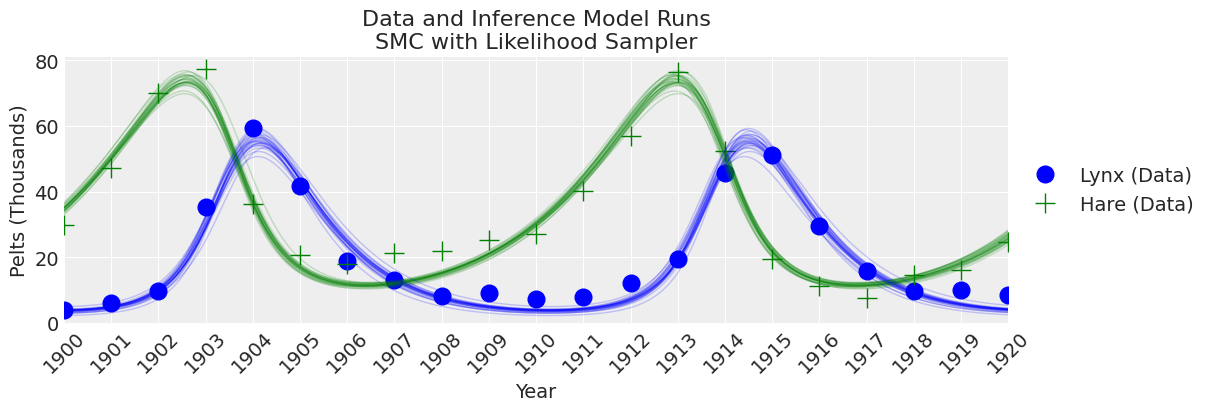
../../../_images/38d3a0e5443b5b8fc84c574e90ed252a08817808cbfbdade625e1d239f5e2cae.png

注释：
在此样本数量和调优方案下，SMC算法相比于其他采样器产生了更宽的不确定性界限。

使用 `pm.Simulator` Epsilon=1#

如PyMC.io上的SMC教程所述，SMC采样器可用于近似贝叶斯计算，即我们可以使用pm.Simulator而不是显式似然。以下是PyMC - odeint模型为SMC-ABC的重写。

模拟器函数需要具有正确的签名（例如，首先接受一个rng参数）。

# simulator function based on the signature rng, parameters, size.
def simulator_forward_model(rng, alpha, beta, gamma, delta, xt0, yt0, sigma, size=None):
    theta = alpha, beta, gamma, delta, xt0, yt0
    mu = odeint(func=rhs, y0=theta[-2:], t=data.year, args=(theta,))
    return rng.normal(mu, sigma)

这里是带有模拟器函数的模型。与显式似然函数不同，模拟器使用距离度量（默认为高斯）来比较模拟值和观测值之间的差异。使用模拟器时，我们还需要指定epsilon，即模拟值和观测值之间差异的容差值。如果epsilon过低，SMC将无法从初始值或少数值中移动。我们可以通过az.plot_trace轻松地看到这一点。如果epsilon过高，后验将几乎等同于先验。因此

with pm.Model() as model:
    # Specify prior distributions for model parameters
    alpha = pm.TruncatedNormal("alpha", mu=theta[0], sigma=0.1, lower=0, initval=theta[0])
    beta = pm.TruncatedNormal("beta", mu=theta[1], sigma=0.01, lower=0, initval=theta[1])
    gamma = pm.TruncatedNormal("gamma", mu=theta[2], sigma=0.1, lower=0, initval=theta[2])
    delta = pm.TruncatedNormal("delta", mu=theta[3], sigma=0.01, lower=0, initval=theta[3])
    xt0 = pm.TruncatedNormal("xto", mu=theta[4], sigma=1, lower=0, initval=theta[4])
    yt0 = pm.TruncatedNormal("yto", mu=theta[5], sigma=1, lower=0, initval=theta[5])
    sigma = pm.HalfNormal("sigma", 10)

    # ode_solution
    pm.Simulator(
        "Y_obs",
        simulator_forward_model,
        params=(alpha, beta, gamma, delta, xt0, yt0, sigma),
        epsilon=1,
        observed=data[["hare", "lynx"]].values,
    )

推理。注意 progressbar 抛出了一个错误，因此它被关闭了。

sampler = "SMC_epsilon=1"
draws = 2000
with model:
    trace_SMC_e1 = pm.sample_smc(draws=draws, progressbar=False)
trace = trace_SMC_e1
az.summary(trace)

Initializing SMC sampler...
Sampling 4 chains in 4 jobs

The rhat statistic is larger than 1.01 for some parameters. This indicates problems during sampling. See https://arxiv.org/abs/1903.08008 for details
The effective sample size per chain is smaller than 100 for some parameters.  A higher number is needed for reliable rhat and ess computation. See https://arxiv.org/abs/1903.08008 for details

	mean	sd	hdi_3%	hdi_97%	mcse_mean	mcse_sd	ess_bulk	ess_tail	r_hat
alpha	0.474	0.012	0.460	0.492	0.006	0.004	5.0	5.0	3.41
beta	0.024	0.000	0.024	0.025	0.000	0.000	5.0	4.0	4.01
gamma	0.946	0.023	0.918	0.986	0.011	0.008	4.0	4.0	3.43
delta	0.028	0.001	0.028	0.029	0.000	0.000	4.0	4.0	4.19
xto	34.734	0.582	33.747	35.194	0.289	0.221	4.0	4.0	7.21
yto	3.814	0.214	3.429	3.966	0.101	0.077	4.0	5.0	3.93
sigma	1.899	0.357	1.369	2.206	0.173	0.132	4.0	8000.0	4.65

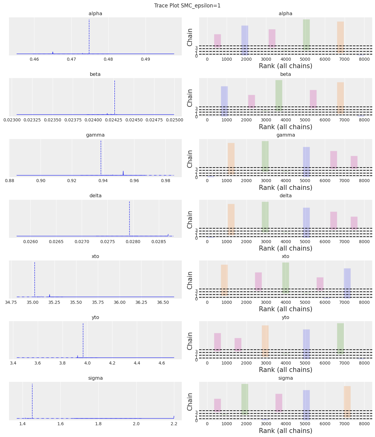
az.plot_trace(trace, kind="rank_bars")
plt.suptitle(f"Trace Plot {sampler}");

/home/osvaldo/proyectos/00_BM/arviz/arviz/stats/density_utils.py:487: UserWarning: Your data appears to have a single value or no finite values
  warnings.warn("Your data appears to have a single value or no finite values")

../../../_images/62c325828bf98319a28883e497373eba5dff17200096f36f89f3740869f2b77c.png

fig, ax = plt.subplots(figsize=(12, 4))
plot_inference(ax, trace, title=f"Data and Inference Model Runs\n{sampler} Sampler");

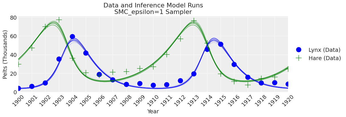
../../../_images/d89c12b874f28ae6ad625f7ca407509a86d8f9eec7be58e063909f747af22811.png

注意：
我们可以看到，如果epsilon太低，plot_trace将会清楚地显示出来。

SMC with Epsilon = 10#

with pm.Model() as model:
    # Specify prior distributions for model parameters
    alpha = pm.TruncatedNormal("alpha", mu=theta[0], sigma=0.1, lower=0, initval=theta[0])
    beta = pm.TruncatedNormal("beta", mu=theta[1], sigma=0.01, lower=0, initval=theta[1])
    gamma = pm.TruncatedNormal("gamma", mu=theta[2], sigma=0.1, lower=0, initval=theta[2])
    delta = pm.TruncatedNormal("delta", mu=theta[3], sigma=0.01, lower=0, initval=theta[3])
    xt0 = pm.TruncatedNormal("xto", mu=theta[4], sigma=1, lower=0, initval=theta[4])
    yt0 = pm.TruncatedNormal("yto", mu=theta[5], sigma=1, lower=0, initval=theta[5])
    sigma = pm.HalfNormal("sigma", 10)

    # ode_solution
    pm.Simulator(
        "Y_obs",
        simulator_forward_model,
        params=(alpha, beta, gamma, delta, xt0, yt0, sigma),
        epsilon=10,
        observed=data[["hare", "lynx"]].values,
    )

sampler = "SMC epsilon=10"
draws = 2000
with model:
    trace_SMC_e10 = pm.sample_smc(draws=draws)
trace = trace_SMC_e10
az.summary(trace)

Initializing SMC sampler...
Sampling 4 chains in 4 jobs

100.00% [100/100 00:00<? Stage: 5 Beta: 1.000]

	mean	sd	hdi_3%	hdi_97%	mcse_mean	mcse_sd	ess_bulk	ess_tail	r_hat
alpha	0.483	0.035	0.416	0.548	0.000	0.000	7612.0	7414.0	1.0
beta	0.025	0.003	0.020	0.030	0.000	0.000	7222.0	7768.0	1.0
gamma	0.927	0.072	0.795	1.063	0.001	0.001	7710.0	7361.0	1.0
delta	0.028	0.002	0.023	0.032	0.000	0.000	7782.0	7565.0	1.0
xto	34.888	0.965	33.145	36.781	0.011	0.008	7921.0	7521.0	1.0
yto	3.902	0.723	2.594	5.319	0.008	0.006	7993.0	7835.0	1.0
sigma	1.450	1.080	0.024	3.409	0.013	0.009	7490.0	7172.0	1.0

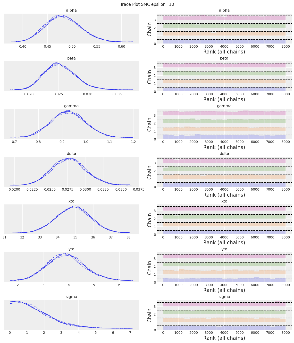
az.plot_trace(trace, kind="rank_bars")
plt.suptitle(f"Trace Plot {sampler}");

../../../_images/0f88f45d3285cea7668b97c7bbf082e520f6613e53ea7d3708cc19d8d82bcfdb.png

fig, ax = plt.subplots(figsize=(12, 4))
plot_inference(ax, trace, title=f"Data and Inference Model Runs\n{sampler} Sampler");

../../../_images/3e34ac526c0f73e61a4d017aba38c36cfec24d11a8084b72fe4b09659c59780c.png

注释：
现在我们为epsilon设置了一个较大的值，可以看到SMC采样器（加上模拟器）提供了良好的结果。选择epsilon的值总是需要一些尝试和错误。那么，在实践中该怎么做呢？由于epsilon是距离函数的尺度。如果你对模拟值和观测值之间的误差没有概念，那么选择epsilon的初始猜测的一个经验法则是使用一个比观测数据的标准差小的数字，可能小一个数量级左右。

后验相关性#

顺便提一下，值得指出的是，后验参数空间对于采样来说是一个困难的拓扑结构。

az.plot_pair(trace_DEM, figsize=(8, 6), scatter_kwargs=dict(alpha=0.01), marginals=True)
plt.suptitle("Pair Plot Showing Posterior Correlations", size=18);

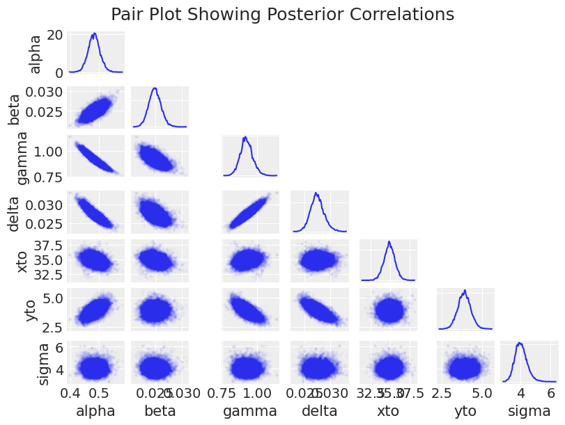
../../../_images/1d4365caf7f9bd2608ebed51cee8e55ba7fc727c43961e5a4297ca70f59d52a2.png

这里的主要观察结果是，后验形状对于采样器来说非常难以处理，具有正相关、负相关、新月形状以及尺度上的巨大变化。这导致了采样速度缓慢（除了求解ODE数千次带来的计算开销）。这也是一个有趣的观察点，有助于理解模型参数之间的相互影响。

带有梯度的贝叶斯推断#

NUTS，PyMC 默认的采样器，只能在向采样器提供梯度的情况下使用。在本节中，我们将通过两种不同的方式在 PyMC 中求解 ODE 系统，这两种方式都向采样器提供了梯度。第一种是内置的 pymc.ode.DifferentialEquation 求解器，第二种是使用 pytensor.scan 进行前向模拟，这允许循环。请注意，可能还有其他更好、更快的使用梯度进行 ODE 贝叶斯推断的方法，例如 sunode 项目，以及依赖于 JAX 的 diffrax。

PyMC ODE 模块#

Pymc.ode 在底层使用 scipy.odeint 来估计解，然后通过有限差分估计梯度。

pymc.ode API 类似于 scipy.odeint。右侧方程放在一个函数中，并写成如果 y 和 p 是向量的形式，如下所示。（即使您的模型有一个状态和/或一个参数，您也应该明确地写成 y[0] 和/或 p[0]。）

def rhs_pymcode(y, t, p):
    dX_dt = p[0] * y[0] - p[1] * y[0] * y[1]
    dY_dt = -p[2] * y[1] + p[3] * y[0] * y[1]
    return [dX_dt, dY_dt]

DifferentialEquation 接受以下参数：

func: 指定微分方程的函数（即 \(f(\mathbf{y},t,\mathbf{p})\)），
times: 数据被观测的时间数组，
n_states: \(f(\mathbf{y},t,\mathbf{p})\) 的维度（输出参数的数量），
n_theta: \(\mathbf{p}\) 的维度（输入参数的数量），
t0: 可选的时间，表示初始条件所属的时间，

如下：

ode_model = DifferentialEquation(
    func=rhs_pymcode, times=data.year.values, n_states=2, n_theta=4, t0=data.year.values[0]
)

一旦常微分方程（ODE）被指定，我们就可以在PyMC模型中使用它。

使用NUTS进行推理#

pymc.ode 相当慢，因此为了演示目的，我们只会抽取少量样本。

with pm.Model() as model:
    # Priors
    alpha = pm.TruncatedNormal("alpha", mu=theta[0], sigma=0.1, lower=0, initval=theta[0])
    beta = pm.TruncatedNormal("beta", mu=theta[1], sigma=0.01, lower=0, initval=theta[1])
    gamma = pm.TruncatedNormal("gamma", mu=theta[2], sigma=0.1, lower=0, initval=theta[2])
    delta = pm.TruncatedNormal("delta", mu=theta[3], sigma=0.01, lower=0, initval=theta[3])
    xt0 = pm.TruncatedNormal("xto", mu=theta[4], sigma=1, lower=0, initval=theta[4])
    yt0 = pm.TruncatedNormal("yto", mu=theta[5], sigma=1, lower=0, initval=theta[5])
    sigma = pm.HalfNormal("sigma", 10)

    # ode_solution
    ode_solution = ode_model(y0=[xt0, yt0], theta=[alpha, beta, gamma, delta])

    # Likelihood
    pm.Normal("Y_obs", mu=ode_solution, sigma=sigma, observed=data[["hare", "lynx"]].values)

sampler = "NUTS PyMC ODE"
tune = draws = 15
with model:
    trace_pymc_ode = pm.sample(tune=tune, draws=draws)

Only 15 samples in chain.
Auto-assigning NUTS sampler...
Initializing NUTS using jitter+adapt_diag...
Multiprocess sampling (4 chains in 4 jobs)
NUTS: [alpha, beta, gamma, delta, xto, yto, sigma]

100.00% [120/120 00:59<00:00 Sampling 4 chains, 0 divergences]

 lsoda--  warning..internal t (=r1) and h (=r2) are       such that in the machine, t + h = t on the next step  
       (h = step size). solver will continue anyway      in above,  r1 =  0.1900000000000D+04   r2 =  0.2340415876362D-14
 lsoda--  warning..internal t (=r1) and h (=r2) are       such that in the machine, t + h = t on the next step  
       (h = step size). solver will continue anyway      in above,  r1 =  0.1900000000000D+04   r2 =  0.2340415876362D-14

/home/osvaldo/anaconda3/envs/pymc/lib/python3.10/site-packages/scipy/integrate/_odepack_py.py:248: ODEintWarning: Excess work done on this call (perhaps wrong Dfun type). Run with full_output = 1 to get quantitative information.
  warnings.warn(warning_msg, ODEintWarning)

 lsoda--  warning..internal t (=r1) and h (=r2) are       such that in the machine, t + h = t on the next step  
       (h = step size). solver will continue anyway      in above,  r1 =  0.1900000000000D+04   r2 =  0.7324477632756D-17
 lsoda--  warning..internal t (=r1) and h (=r2) are       such that in the machine, t + h = t on the next step  
       (h = step size). solver will continue anyway      in above,  r1 =  0.1900000000000D+04   r2 =  0.5527744901481D-17
 lsoda--  warning..internal t (=r1) and h (=r2) are       such that in the machine, t + h = t on the next step  
       (h = step size). solver will continue anyway      in above,  r1 =  0.1900000000000D+04   r2 =  0.1105548980296D-16
 lsoda--  warning..internal t (=r1) and h (=r2) are       such that in the machine, t + h = t on the next step  
       (h = step size). solver will continue anyway      in above,  r1 =  0.1900000000000D+04   r2 =  0.1105548980296D-16
 lsoda--  warning..internal t (=r1) and h (=r2) are       such that in the machine, t + h = t on the next step  
       (h = step size). solver will continue anyway      in above,  r1 =  0.1900000000000D+04   r2 =  0.1105548980296D-16
 lsoda--  warning..internal t (=r1) and h (=r2) are       such that in the machine, t + h = t on the next step  
       (h = step size). solver will continue anyway      in above,  r1 =  0.1900000000000D+04   r2 =  0.1105548980296D-15
 lsoda--  warning..internal t (=r1) and h (=r2) are       such that in the machine, t + h = t on the next step  
       (h = step size). solver will continue anyway      in above,  r1 =  0.1900000000000D+04   r2 =  0.1105548980296D-15
 lsoda--  warning..internal t (=r1) and h (=r2) are       such that in the machine, t + h = t on the next step  
       (h = step size). solver will continue anyway      in above,  r1 =  0.1900000000000D+04   r2 =  0.1105548980296D-15
 lsoda--  warning..internal t (=r1) and h (=r2) are       such that in the machine, t + h = t on the next step  
       (h = step size). solver will continue anyway      in above,  r1 =  0.1900000000000D+04   r2 =  0.1105548980296D-15
 lsoda--  warning..internal t (=r1) and h (=r2) are       such that in the machine, t + h = t on the next step  
       (h = step size). solver will continue anyway      in above,  r1 =  0.1900000000000D+04   r2 =  0.1105548980296D-14
 lsoda--  above warning has been issued i1 times.         it will not be issued again for this problem      in above message,  i1 =        10
 lsoda--  warning..internal t (=r1) and h (=r2) are       such that in the machine, t + h = t on the next step  
       (h = step size). solver will continue anyway      in above,  r1 =  0.1900000000000D+04   r2 =  0.5241493348134D-15
 lsoda--  warning..internal t (=r1) and h (=r2) are       such that in the machine, t + h = t on the next step  
       (h = step size). solver will continue anyway      in above,  r1 =  0.1900000000000D+04   r2 =  0.5241493348134D-15
 lsoda--  warning..internal t (=r1) and h (=r2) are       such that in the machine, t + h = t on the next step  
       (h = step size). solver will continue anyway      in above,  r1 =  0.1900000000000D+04   r2 =  0.1088694571877D-13
 lsoda--  warning..internal t (=r1) and h (=r2) are       such that in the machine, t + h = t on the next step  
       (h = step size). solver will continue anyway      in above,  r1 =  0.1900000000000D+04   r2 =  0.1088694571877D-13
 lsoda--  warning..internal t (=r1) and h (=r2) are       such that in the machine, t + h = t on the next step  
       (h = step size). solver will continue anyway      in above,  r1 =  0.1900000000000D+04   r2 =  0.1088694571877D-13
 lsoda--  warning..internal t (=r1) and h (=r2) are       such that in the machine, t + h = t on the next step  
       (h = step size). solver will continue anyway      in above,  r1 =  0.1900000000000D+04   r2 =  0.4463323525725D-13
 lsoda--  warning..internal t (=r1) and h (=r2) are       such that in the machine, t + h = t on the next step  
       (h = step size). solver will continue anyway      in above,  r1 =  0.1900000000000D+04   r2 =  0.3388355031231D-13
 lsoda--  warning..internal t (=r1) and h (=r2) are       such that in the machine, t + h = t on the next step  
       (h = step size). solver will continue anyway      in above,  r1 =  0.1900000000000D+04   r2 =  0.3388355031231D-13
 lsoda--  warning..internal t (=r1) and h (=r2) are       such that in the machine, t + h = t on the next step  
       (h = step size). solver will continue anyway      in above,  r1 =  0.1900000000000D+04   r2 =  0.3388355031231D-13
 lsoda--  warning..internal t (=r1) and h (=r2) are       such that in the machine, t + h = t on the next step  
       (h = step size). solver will continue anyway      in above,  r1 =  0.1900000000000D+04   r2 =  0.6776710062462D-13
 lsoda--  above warning has been issued i1 times.         it will not be issued again for this problem      in above message,  i1 =        10
 lsoda--  warning..internal t (=r1) and h (=r2) are       such that in the machine, t + h = t on the next step  
       (h = step size). solver will continue anyway      in above,  r1 =  0.1900000000000D+04   r2 =  0.4158457835953D-42
 lsoda--  warning..internal t (=r1) and h (=r2) are       such that in the machine, t + h = t on the next step  
       (h = step size). solver will continue anyway      in above,  r1 =  0.1900000000000D+04   r2 =  0.4158457835953D-42
 lsoda--  warning..internal t (=r1) and h (=r2) are       such that in the machine, t + h = t on the next step  
       (h = step size). solver will continue anyway      in above,  r1 =  0.1900000000000D+04   r2 =  0.1370912617246D-40
 lsoda--  warning..internal t (=r1) and h (=r2) are       such that in the machine, t + h = t on the next step  
       (h = step size). solver will continue anyway      in above,  r1 =  0.1900000000000D+04   r2 =  0.1370912617246D-40
 lsoda--  warning..internal t (=r1) and h (=r2) are       such that in the machine, t + h = t on the next step  
       (h = step size). solver will continue anyway      in above,  r1 =  0.1900000000000D+04   r2 =  0.1370912617246D-40
 lsoda--  warning..internal t (=r1) and h (=r2) are       such that in the machine, t + h = t on the next step  
       (h = step size). solver will continue anyway      in above,  r1 =  0.1900000000000D+04   r2 =  0.5948148309049D-40
 lsoda--  warning..internal t (=r1) and h (=r2) are       such that in the machine, t + h = t on the next step  
       (h = step size). solver will continue anyway      in above,  r1 =  0.1900000000000D+04   r2 =  0.4374718724784D-40
 lsoda--  warning..internal t (=r1) and h (=r2) are       such that in the machine, t + h = t on the next step  
       (h = step size). solver will continue anyway      in above,  r1 =  0.1900000000000D+04   r2 =  0.3628059832750D-40
 lsoda--  warning..internal t (=r1) and h (=r2) are       such that in the machine, t + h = t on the next step  
       (h = step size). solver will continue anyway      in above,  r1 =  0.1900000000000D+04   r2 =  0.3628059832750D-40
 lsoda--  warning..internal t (=r1) and h (=r2) are       such that in the machine, t + h = t on the next step  
       (h = step size). solver will continue anyway      in above,  r1 =  0.1900000000000D+04   r2 =  0.3628059832750D-40
 lsoda--  above warning has been issued i1 times.         it will not be issued again for this problem      in above message,  i1 =        10

/home/osvaldo/anaconda3/envs/pymc/lib/python3.10/site-packages/scipy/integrate/_odepack_py.py:248: ODEintWarning: Excess work done on this call (perhaps wrong Dfun type). Run with full_output = 1 to get quantitative information.
  warnings.warn(warning_msg, ODEintWarning)
/home/osvaldo/anaconda3/envs/pymc/lib/python3.10/site-packages/scipy/integrate/_odepack_py.py:248: ODEintWarning: Excess work done on this call (perhaps wrong Dfun type). Run with full_output = 1 to get quantitative information.
  warnings.warn(warning_msg, ODEintWarning)

 lsoda--  warning..internal t (=r1) and h (=r2) are       such that in the machine, t + h = t on the next step  
       (h = step size). solver will continue anyway      in above,  r1 =  0.1900000000000D+04   r2 =  0.8146615298522D-82
 lsoda--  warning..internal t (=r1) and h (=r2) are       such that in the machine, t + h = t on the next step  
       (h = step size). solver will continue anyway      in above,  r1 =  0.1900000000000D+04   r2 =  0.8146615298522D-82
 lsoda--  warning..internal t (=r1) and h (=r2) are       such that in the machine, t + h = t on the next step  
       (h = step size). solver will continue anyway      in above,  r1 =  0.1900000000000D+04   r2 =  0.8146615298522D-78
 lsoda--  warning..internal t (=r1) and h (=r2) are       such that in the machine, t + h = t on the next step  
       (h = step size). solver will continue anyway      in above,  r1 =  0.1900000000000D+04   r2 =  0.8146615298522D-78
 lsoda--  warning..internal t (=r1) and h (=r2) are       such that in the machine, t + h = t on the next step  
       (h = step size). solver will continue anyway      in above,  r1 =  0.1900000000000D+04   r2 =  0.8146615298522D-78
 lsoda--  warning..internal t (=r1) and h (=r2) are       such that in the machine, t + h = t on the next step  
       (h = step size). solver will continue anyway      in above,  r1 =  0.1900000000000D+04   r2 =  0.8146615298522D-77
 lsoda--  warning..internal t (=r1) and h (=r2) are       such that in the machine, t + h = t on the next step  
       (h = step size). solver will continue anyway      in above,  r1 =  0.1900000000000D+04   r2 =  0.8146615298522D-77
 lsoda--  warning..internal t (=r1) and h (=r2) are       such that in the machine, t + h = t on the next step  
       (h = step size). solver will continue anyway      in above,  r1 =  0.1900000000000D+04   r2 =  0.8146615298522D-77
 lsoda--  warning..internal t (=r1) and h (=r2) are       such that in the machine, t + h = t on the next step  
       (h = step size). solver will continue anyway      in above,  r1 =  0.1900000000000D+04   r2 =  0.8146615298522D-77
 lsoda--  warning..internal t (=r1) and h (=r2) are       such that in the machine, t + h = t on the next step  
       (h = step size). solver will continue anyway      in above,  r1 =  0.1900000000000D+04   r2 =  0.7775771408140D-76
 lsoda--  above warning has been issued i1 times.         it will not be issued again for this problem      in above message,  i1 =        10

Sampling 4 chains for 15 tune and 15 draw iterations (60 + 60 draws total) took 60 seconds.
The number of samples is too small to check convergence reliably.

trace = trace_pymc_ode
az.summary(trace)

	mean	sd	hdi_3%	hdi_97%	mcse_mean	mcse_sd	ess_bulk	ess_tail	r_hat
alpha	0.472	0.031	0.389	0.506	0.008	0.006	17.0	33.0	1.36
beta	0.026	0.003	0.022	0.032	0.001	0.001	12.0	40.0	1.54
gamma	0.959	0.080	0.868	1.151	0.025	0.018	11.0	33.0	1.59
delta	0.029	0.003	0.026	0.035	0.001	0.001	14.0	37.0	1.33
xto	34.907	0.852	33.526	36.300	0.099	0.071	98.0	43.0	1.21
yto	3.347	0.772	1.742	4.342	0.278	0.205	10.0	16.0	1.78
sigma	6.117	4.425	3.502	16.420	1.353	0.984	9.0	16.0	1.87

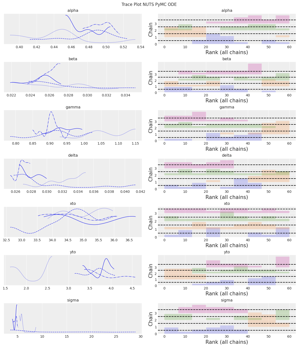
az.plot_trace(trace, kind="rank_bars")
plt.suptitle(f"Trace Plot {sampler}");

../../../_images/865e2a14c2c8b3d05fccf1a4a15da05da5b37709efe754f73b7475414da11b5e.png

_, ax = plt.subplots(figsize=(12, 4))
plot_inference(ax, trace, title=f"Data and Inference Model Runs\n{sampler} Sampler");

../../../_images/63ccdef49b1a0027e96f2f47e698850599c5fef8f831d9f4a5b8fdeaae37952b.png

注意：
NUTS 开始找到正确的后验分布，但需要更多的时间来进行良好的推断。

使用 Pytensor Scan 进行模拟#

最后，我们可以在PyMC中将ODE系统写成一个前向模拟求解器。在PyMC中编写for循环的方法是使用pytensor.scan。然后通过自动微分将梯度提供给采样器。

首先，我们应该测试时间步长是否足够小，以获得合理的估计。

检查时间步#

创建一个函数，该函数接受不同数量的时间步长用于测试。该函数还演示了如何使用pytensor.scan。

# Lotka-Volterra forward simulation model using scan
def lv_scan_simulation_model(theta, steps_year=100, years=21):
    # variables to control time steps
    n_steps = years * steps_year
    dt = 1 / steps_year

    # PyMC model
    with pm.Model() as model:
        # Priors (these are static for testing)
        alpha = theta[0]
        beta = theta[1]
        gamma = theta[2]
        delta = theta[3]
        xt0 = theta[4]
        yt0 = theta[5]

        # Lotka-Volterra calculation function
        ## Similar to the right-hand-side functions used earlier
        ## but with dt applied to the equations
        def ode_update_function(x, y, alpha, beta, gamma, delta):
            x_new = x + (alpha * x - beta * x * y) * dt
            y_new = y + (-gamma * y + delta * x * y) * dt
            return x_new, y_new

        # Pytensor scan looping function
        ## The function argument names are not intuitive in this context!
        result, updates = pytensor.scan(
            fn=ode_update_function,  # function
            outputs_info=[xt0, yt0],  # initial conditions
            non_sequences=[alpha, beta, gamma, delta],  # parameters
            n_steps=n_steps,  # number of loops
        )

        # Put the results together and track the result
        pm.Deterministic("result", pm.math.stack([result[0], result[1]], axis=1))

    return model

运行模拟以获取不同时间步长的结果并绘制结果。

_, ax = plt.subplots(figsize=(12, 4))

steps_years = [12, 100, 1000, 10000]
for steps_year in steps_years:
    time = np.arange(1900, 1921, 1 / steps_year)
    model = lv_scan_simulation_model(theta, steps_year=steps_year)
    with model:
        prior = pm.sample_prior_predictive(1)
    ax.plot(time, prior.prior.result[0][0].values, label=str(steps_year) + " steps/year")
ax.legend(loc="center left", bbox_to_anchor=(1, 0.5))
ax.set_title("Lotka-Volterra Forward Simulation Model with different step sizes");

Sampling: []
Sampling: []
Sampling: []
Sampling: []

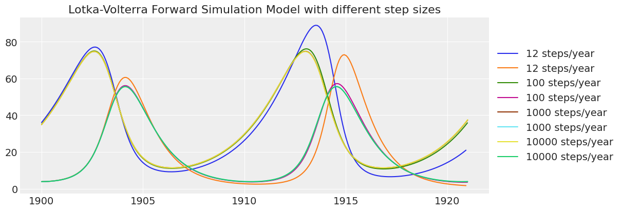
../../../_images/7fe7cb4865ce60723cb29960f65a5c071493cb587df84e4af670fd1e82a8094a.png

请注意，低分辨率的模拟随着时间的推移准确性较低。根据这一检查，每年100个时间步长已足够准确。每年12个时间步长在20年的模拟中会产生过多的“数值扩散”。

使用NUTs进行推理#

既然我们每年有100个时间步长是可以接受的，我们编写模型时使用索引来使数据与结果对齐。

def lv_scan_inference_model(theta, steps_year=100, years=21):
    # variables to control time steps
    n_steps = years * steps_year
    dt = 1 / steps_year

    # variables to control indexing to get annual values
    segment = [True] + [False] * (steps_year - 1)
    boolist_idxs = []
    for _ in range(years):
        boolist_idxs += segment

    # PyMC model
    with pm.Model() as model:
        # Priors
        alpha = pm.TruncatedNormal("alpha", mu=theta[0], sigma=0.1, lower=0, initval=theta[0])
        beta = pm.TruncatedNormal("beta", mu=theta[1], sigma=0.01, lower=0, initval=theta[1])
        gamma = pm.TruncatedNormal("gamma", mu=theta[2], sigma=0.1, lower=0, initval=theta[2])
        delta = pm.TruncatedNormal("delta", mu=theta[3], sigma=0.01, lower=0, initval=theta[3])
        xt0 = pm.TruncatedNormal("xto", mu=theta[4], sigma=1, lower=0, initval=theta[4])
        yt0 = pm.TruncatedNormal("yto", mu=theta[5], sigma=1, lower=0, initval=theta[5])
        sigma = pm.HalfNormal("sigma", 10)

        # Lotka-Volterra calculation function
        def ode_update_function(x, y, alpha, beta, gamma, delta):
            x_new = x + (alpha * x - beta * x * y) * dt
            y_new = y + (-gamma * y + delta * x * y) * dt
            return x_new, y_new

        # Pytensor scan is a looping function
        result, updates = pytensor.scan(
            fn=ode_update_function,  # function
            outputs_info=[xt0, yt0],  # initial conditions
            non_sequences=[alpha, beta, gamma, delta],  # parameters
            n_steps=n_steps,
        )  # number of loops

        # Put the results together
        final_result = pm.math.stack([result[0], result[1]], axis=1)
        # Filter the results down to annual values
        annual_value = final_result[np.array(boolist_idxs), :]

        # Likelihood function
        pm.Normal("Y_obs", mu=annual_value, sigma=sigma, observed=data[["hare", "lynx"]].values)
    return model

这也非常慢，因此我们只拉取一些样本用于演示目的。

steps_year = 100
model = lv_scan_inference_model(theta, steps_year=steps_year)
sampler = "NUTS Pytensor Scan"
tune = draws = 50
with model:
    trace_scan = pm.sample(tune=tune, draws=draws)

Only 50 samples in chain.
Auto-assigning NUTS sampler...
Initializing NUTS using jitter+adapt_diag...
Multiprocess sampling (4 chains in 4 jobs)
NUTS: [alpha, beta, gamma, delta, xto, yto, sigma]

100.00% [400/400 01:29<00:00 Sampling 4 chains, 0 divergences]

Sampling 4 chains for 50 tune and 50 draw iterations (200 + 200 draws total) took 89 seconds.
The number of samples is too small to check convergence reliably.

trace = trace_scan
az.summary(trace)

	mean	sd	hdi_3%	hdi_97%	mcse_mean	mcse_sd	ess_bulk	ess_tail	r_hat
alpha	0.480	0.025	0.432	0.526	0.003	0.002	77.0	94.0	1.02
beta	0.025	0.001	0.023	0.027	0.000	0.000	147.0	155.0	1.03
gamma	0.933	0.054	0.832	1.030	0.007	0.005	70.0	80.0	1.04
delta	0.028	0.002	0.024	0.031	0.000	0.000	70.0	94.0	1.04
xto	34.877	0.764	33.232	36.118	0.046	0.032	265.0	110.0	1.04
yto	3.987	0.504	2.887	4.749	0.069	0.049	58.0	102.0	1.06
sigma	4.173	0.488	3.361	5.005	0.056	0.039	83.0	104.0	1.03

az.plot_trace(trace, kind="rank_bars")
plt.suptitle(f"Trace Plot {sampler}");

../../../_images/8630144f98555b60164b9b54851b5b1141ae549ccb22802037805ce1d7a6564d.png

time = np.arange(1900, 1921, 0.01)
odeint(func=rhs, y0=theta[-2:], t=time, args=(theta,)).shape

(2100, 2)

_, ax = plt.subplots(figsize=(12, 4))
plot_inference(ax, trace, title=f"Data and Inference Model Runs\n{sampler} Sampler");

../../../_images/e7982c055cc693d6b1cd80f885d5100d03c6f1b5c9f38fd33a17a278c2654b50.png

注意：
采样器比pymc.ode实现更快，但仍然比结合无梯度推断方法的scipy odeint慢。

概述#

让我们比较一下这些不同方法的推理结果。请记住，为了在合理的时间内运行此笔记本，我们对许多推理方法的样本数量不足。为了进行公平比较，我们需要增加样本数量并延长笔记本的运行时间。尽管如此，我们还是来看一下。

# Make lists with variable for looping
var_names = [str(s).split("_")[0] for s in list(model.values_to_rvs.keys())[:-1]]
# Make lists with model results and model names for plotting
inference_results = [
    trace_slice,
    trace_DEMZ,
    trace_DEM,
    trace_M,
    trace_SMC_like,
    trace_SMC_e1,
    trace_SMC_e10,
    trace_pymc_ode,
    trace_scan,
]
model_names = [
    "Slice Sampler",
    "DEMetropolisZ",
    "DEMetropolis",
    "Metropolis",
    "SMC with Likelihood",
    "SMC e=1",
    "SMC e=10",
    "PyMC ODE NUTs",
    "Pytensor Scan NUTs",
]

# Loop through variable names
for var_name in var_names:
    axes = az.plot_forest(
        inference_results,
        model_names=model_names,
        var_names=var_name,
        kind="forestplot",
        legend=False,
        combined=True,
        figsize=(7, 3),
    )
    axes[0].set_title(f"Marginal Probability: {var_name}")
    # Clean up ytick labels
    ylabels = axes[0].get_yticklabels()
    new_ylabels = []
    for label in ylabels:
        txt = label.get_text()
        txt = txt.replace(": " + var_name, "")
        label.set_text(txt)
        new_ylabels.append(label)
    axes[0].set_yticklabels(new_ylabels)

    plt.show();

../../../_images/4656ec630fb0303ff1c51e0638c1d0b408b05aa3c0a9737ba9023f2cc58c5b03.png

../../../_images/74171cf0001650514775294ba6fc367310b23d48ca8fa05f17ac2b2de8b493b7.png

../../../_images/009a9d6a1ab98c6e57ea434698e85bc150b65ef3ddb754443fb0d0d8e2b3e66d.png

../../../_images/cfd13e4bc43b8d56327fbba949cdcf9a14508009a92cdca08190713d3a890a54.png

../../../_images/c2f6f95168da0b282e5c49de0ffff62aacf307f5421cdaf8122efe36ddefa443.png

../../../_images/4e06d4fc0a7acab074926d27dba2de9fd5c02c097a253368c296047b98218322.png

../../../_images/48431a06e37309cb284a0f4e19552189a15aff23242a2c6b7b6e926cbfac0daf.png

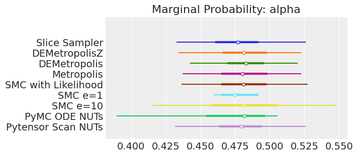
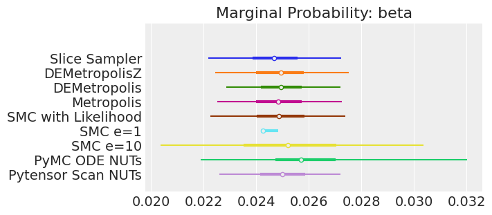
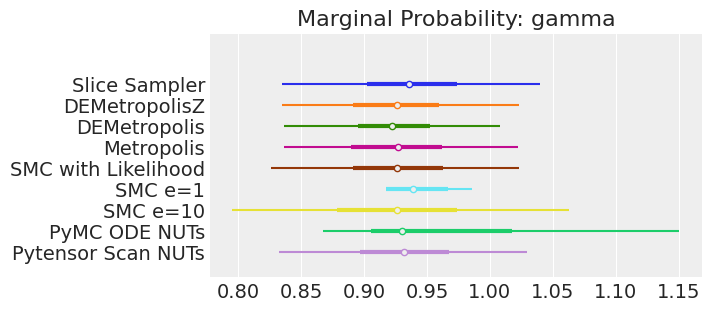
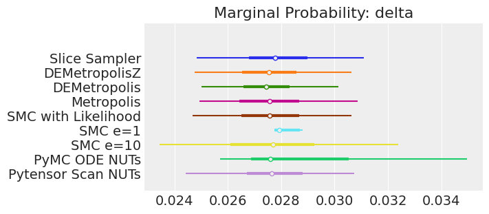
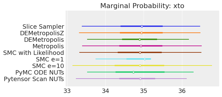
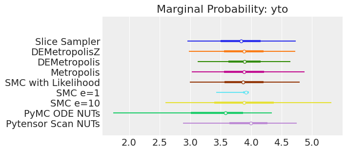
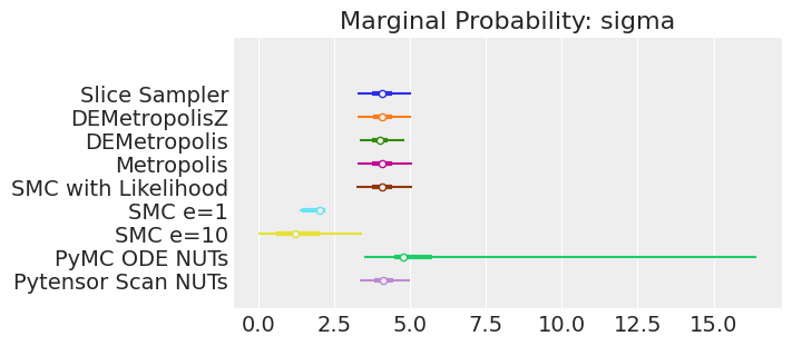
注释：
如果我们运行采样器足够长的时间以获得良好的推断，我们预计它们会收敛到相同的后验概率分布。对于近似贝叶斯计算（Approximate Bayesian Computation），除非我们首先确保似然度的近似足够好，否则这不一定成立。例如，SMCe=1给出了错误的结果，我们一直在警告，当我们使用plot_trace作为诊断时，这种情况很可能是这样的。对于SMC e=10，我们看到后验均值与其他采样器一致，但后验分布更宽。这是ABC方法所预期的。较小的epsilon值，可能是5，应该提供更接近真实值的后验分布。

关键结论#

我们通过四种主要方式对一组常微分方程系统进行了贝叶斯推断：

Scipy odeint 被封装在一个 Pytensor op 中，并使用非基于梯度的采样器进行采样（比较了5种不同的采样器）。
Scipy odeint 封装在一个 pm.Simulator 函数中，并使用非似然性的顺序蒙特卡罗（SMC）采样器进行采样。
PyMC ode.DifferentialEquation 使用NUTs进行采样。
使用 pytensor.scan 进行前向模拟，并使用 NUTs 进行采样。

这个问题的“获胜者”是Scipy的odeint求解器，结合差分进化（DE）Metropolis采样器和SMC（用于具有似然性的模型）提供了良好的结果，尽管SMC的速度稍慢（但诊断效果更好）。NUTS采样器的改进效率并未能弥补使用带有梯度的慢速ODE求解器时的效率低下。DEMetropolis和SMC都为拥有工作数值模型并希望进行贝叶斯推断的科学家提供了最简单的流程。只需将数值模型包装在Pytensor操作中并将其插入PyMC模型中，就可以走得很远！

作者#

由 Greg Brunkhorst 整理和重写，基于 Sanmitra Ghosh、Demetri Pananos 和 PyMC 团队的多份 PyMC.io 示例笔记本（近似贝叶斯计算）。

Osvaldo Martin 在2023年3月对SMC-ABC进行了一些澄清，并做了一些小的修复

参考资料#

[1]

理查德·麦克埃尔雷思。统计重构：一个带有R和Stan示例的贝叶斯课程。查普曼和霍尔/CRC，2018年。

水印#

%watermark -n -u -v -iv -w

Last updated: Thu Mar 30 2023

Python implementation: CPython
Python version       : 3.10.10
IPython version      : 8.10.0

pytensor  : 2.10.1
pandas    : 1.5.3
matplotlib: 3.5.2
pymc      : 5.1.2+12.g67925df69
numpy     : 1.23.5
arviz     : 0.16.0.dev0

Watermark: 2.3.1

分类

标签

使用多种方法进行贝叶斯推断的ODE Lotka-Volterra#

目的#

关键结论#

背景#

动机#

Lotka-Volterra 捕食者-猎物模型#

哈德逊湾公司数据#

问题陈述#

Scipy `odeint`#

最小二乘解#

无梯度贝叶斯推断的PyMC模型规范#

使用 @as_op 装饰器将 Python 函数转换为 Pytensor 操作符#

PyMC 模型#

绘图函数#

无梯度采样器选项#

切片采样器#

DE MetropolisZ 采样器#

DEMetropolis 采样器#

Metropolis Sampler#

SMC采样器#

带有似然函数的SMC#

使用 `pm.Simulator` Epsilon=1#

SMC with Epsilon = 10#

后验相关性#

带有梯度的贝叶斯推断#

PyMC ODE 模块#

使用NUTS进行推理#

使用 Pytensor Scan 进行模拟#

检查时间步#

使用NUTs进行推理#

概述#

关键结论#

作者#

参考资料#

水印#

分类

标签

使用多种方法进行贝叶斯推断的ODE Lotka-Volterra#

目的#

关键结论#

背景#

动机#

Lotka-Volterra 捕食者-猎物模型#

哈德逊湾公司数据#

问题陈述#

Scipy odeint#

最小二乘解#

无梯度贝叶斯推断的PyMC模型规范#

使用 @as_op 装饰器将 Python 函数转换为 Pytensor 操作符#

PyMC 模型#

绘图函数#

无梯度采样器选项#

切片采样器#

DE MetropolisZ 采样器#

DEMetropolis 采样器#

Metropolis Sampler#

SMC采样器#

带有似然函数的SMC#

使用 pm.Simulator Epsilon=1#

SMC with Epsilon = 10#

后验相关性#

带有梯度的贝叶斯推断#

PyMC ODE 模块#

使用NUTS进行推理#

使用 Pytensor Scan 进行模拟#

检查时间步#

使用NUTs进行推理#

概述#

关键结论#

作者#

参考资料#

水印#

Scipy `odeint`#

使用 `pm.Simulator` Epsilon=1#