


DEMetropolis(Z) 采样器调优#
import time

import arviz as az

az.rcParams["plot.max_subplots"] = 100
import matplotlib.pyplot as plt
import numpy as np
import pandas as pd
import pymc as pm

from matplotlib import cm, gridspec

print(f"Running on PyMC v{pm.__version__}")
WARNING (pytensor.tensor.blas): Using NumPy C-API based implementation for BLAS functions.
Running on PyMC v0+untagged.9358.g8ea092d
%load_ext watermark
az.style.use("arviz-darkgrid")
rng = np.random.default_rng(1234)
背景#
对于连续变量,默认的 PyMC 采样器(NUTS)要求计算梯度,PyMC 通过自动微分来实现这一点。然而,在某些情况下,PyMC 模型可能没有提供梯度(例如,通过在 PyMC 外部评估数值模型),因此需要一个替代的采样器。DEMetropolisZ 采样器是梯度无关推断的高效选择。PyMC 中 DEMetropolisZ 的实现基于 ter Braak 和 Vrugt [2008],但采用了修改后的调优方案。本笔记本比较了采样器的各种调优参数设置,包括在 PyMC 中引入的 drop_tune_fraction 参数。
关键要点 (TL;DR)#
PyMC 中的 DEMetropolisZ 采样器实现具有合理的默认值;然而,在本笔记本中,两个手动调整改善了采样器性能:将 tuning 设置为“scaling”,并将 proposal_dist 设置为 pm.NormalProposal。在最简单的形式中,手动调整如下所示:
with model:
    step = pm.DEMetropolisZ(
        tune='scaling',
        proposal_dist=pm.NormalProposal
    )
    idata = pm.sample(step=step)
采样器方法#
在PyMC中,Metropolis算法对于连续变量的不同变体有不同的方法来决定跳跃的距离和方向。普通的pm.Metropolis采样器执行一个调优过程来调整跳跃的大小。每个跳跃都是从提议分布中随机抽取的值乘以调优后的缩放因子。
差分进化(DE)Metropolis算法使用从其他链中随机选择的抽样(DEMetropolis)或从当前链的过去抽样中(DEMetropolis(Z))进行更明智的跳跃。以下是使用ter Braak和Vrugt [2008]中的命名法进行DEMetropolis算法跳跃的公式:
差分进化跳跃方程#
其中:
\(x^*=\) 提议
\(x_i=\) 当前状态(样本)
\(\gamma=\) 决定跳跃相对于随机向量大小的因子。在PyMC实现中,这被称为
lamb,并且默认情况下会进行调整(起始值为\({2.38}/{\sqrt{2d}}\),其中\(d=\)维度的数量[即参数])。\((x_{R1}-x_{R2})=\) 基于两个随机选择的过去状态(样本)相减得到的随机向量。DEMetropolis 从其他链中选择,而 DEMetropolis(Z) 从当前链的过去抽取中选择。
\(\epsilon=\) 添加到每次移动的额外噪声:
其中:
\(\mathscr{D}_{p}(A)=\) 一个以零为中心的提议分布,方差项为A(在PyMC中默认为A=1的均匀提议分布,即-1到1)。
\(b=\) 缩放因子。这是 PyMC 中的
scaling,可以调整(默认值为 0.001)。
在 PyMC 中,我们可以调整 lamb(\(\gamma\))或 scaling(\(b\)),另一个参数是固定的。
问题陈述#
在本笔记本中,将使用DEMetropolisZ对一个10维的多变量正态目标密度进行采样,同时改变四个参数以识别高效的采样方案。这四个参数如下:
drop_tuning_fraction,它决定了从调优阶段回收的样本数量,用于随机向量\((x_{R1}-x_{R2})\)选择,lamb(\(\gamma\)),用于缩放相对于随机向量的跳跃大小。scaling(\(b\)),用于缩放噪声项\(\epsilon\)的跳跃大小,以及proposal_distribution(\(\mathscr{D}_{p}\)),它决定了从中抽取\(\epsilon\)的形状。
我们将根据三个采样指标来评估这些采样参数:有效样本量、自相关性和样本接受率。
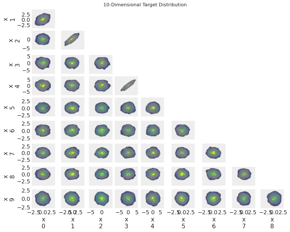
目标分布#
我们使用一个在前几维中具有相关性的多元正态目标密度。函数gen_mvnormal_params生成目标分布的参数。
函数 make_model_sample 接受多元正态参数 mu 和 cov 并输出一个 PyMC 模型和一个目标分布的随机样本。
def make_model_sample(mu, cov, draws=1000):
    with pm.Model() as model:
        x = pm.MvNormal("x", mu=mu, cov=cov, shape=(len(mu),))

    target_sample = pm.draw(x, draws=draws)
    target_idata = az.data.convert_to_inference_data(target_sample[np.newaxis, :], group="target")
    return model, target_idata
示例将是10维的
D = 10
mu, cov = gen_mvnormal_params(D)
model, target_idata = make_model_sample(mu, cov)
c:\Users\greg\.conda\envs\pymc-dev\Lib\site-packages\arviz\data\inference_data.py:153: UserWarning: target group is not defined in the InferenceData scheme
  warnings.warn(
在我们的脑海中有一个分布的图像是很有用的。
az.plot_pair(target_idata.target, kind="kde", figsize=(10, 8))
plt.suptitle("10-Dimensional Target Distribution");
辅助函数#
我们将预先定义一些辅助函数,以便在整个笔记本中重复使用。
采样#
sample_model 执行MCMC,返回轨迹和采样持续时间。
Show code cell source
def sample_model(model, run=0, step_kwargs={}, sample_kwargs={}):
    with model:
        step = pm.DEMetropolisZ(**step_kwargs)
        t_start = time.time()
        idata = pm.sample(
            step=step,
            chains=1,
            initvals={"x": [7.0] * D},
            discard_tuned_samples=False,
            progressbar=False,
            random_seed=2020 + run,
            **sample_kwargs
        )
        t = time.time() - t_start
    return idata, t
MCMC 指标#
为了评估MCMC样本,我们将使用三种不同的指标。
有效样本量 (ESS) 是根据迹中的自相关性调整的样本大小。ESS 将表示为百分比 \({(ESS)}/{(\text{总抽取次数})}*100\)。ESS 越高越好。对于 Metropolis 采样器,2% 的 ESS 已经相当高。
自相关在轨迹中是采样器效率低下的标志,应接近于零。样本100处的自相关(调优后)将用于比较。
接受率在跟踪过程中应大致保持平稳。 接受率下降表明步长一开始设置得太小,而接受率上升则表明步长一开始设置得太大。
calc_ess_pct 计算 \({(ESS)}/{(\text{总抽样次数})}*100\)。
Show code cell source
def calc_ess_pct(idata, chains=1):
    draws = idata.posterior.draw.shape[0] * chains
    ess = az.ess(idata).x.values
    return ess * 100 / draws
calc_autocorr 计算在指定数量的样本后的迹线的自相关性。
Show code cell source
def calc_autocorr(idata, sample=100):
    return az.autocorr(az.extract(idata).x.values)[:, sample]
calc_acceptance 计算迹线的接受率的斜率和截距。
Show code cell source
def calc_acceptance(idata, window=500):
    rolling_rate = (
        pd.Series(idata.sample_stats.accepted.values.flatten()).rolling(window=window).mean().values
    )

    x = np.arange(0, len(rolling_rate))
    A = np.vstack([x, np.ones(len(x))]).T
    slope, intercept = np.linalg.lstsq(A[window - 1 :, :], rolling_rate[window - 1 :], rcond=None)[
        0
    ]

    return slope, intercept, rolling_rate
重复抽样和计算#
sample_model_calc_metrics 对不同参数值的模型进行迭代采样,计算每条轨迹的指标,并返回包含结果的数据框。
Show code cell source
def sample_model_calc_metrics(
    model,
    param="tune_drop_fraction",
    param_values=[0, 0.5, 0.9, 1.0],
    step_kwargs={},
    sample_kwargs={},
    N_tune=10000,
    N_draws=10000,
    N_runs=5,
    window=500,
):
    cols = (param + ",run,ess_pct,autocorr100,accept_slope,time,idata").split(",")
    idx = (param + ",run").split(",")
    df_results = pd.DataFrame(columns=cols).set_index(idx)
    idatas = []
    for param_value in param_values:
        for r in range(N_runs):
            all_step_kwargs = dict(step_kwargs, **{param: param_value})
            idata, t = sample_model(
                model,
                run=r,
                step_kwargs=all_step_kwargs,
                sample_kwargs=dict(sample_kwargs, **dict(tune=N_tune, draws=N_draws)),
            )
            if type(param_value) == type:
                index_name = param_value.__name__[:-8]
            else:
                index_name = param_value
            df_results.loc[(index_name, r), "ess_pct"] = calc_ess_pct(idata).mean()
            df_results.loc[(index_name, r), "autocorr100"] = calc_autocorr(idata).mean()
            slope, _, _ = calc_acceptance(idata, window=window)
            df_results.loc[(index_name, r), "accept_slope"] = slope
            df_results.loc[(index_name, r), "time"] = t
            idatas.append(idata)
    df_results.idata = idatas
    num_cols = ["ess_pct", "autocorr100", "accept_slope", "time"]
    for num_col in num_cols:
        df_results[num_col] = pd.to_numeric(df_results[num_col])
    return df_results
average_results 接受大型结果数据框并对重复运行进行平均。
Show code cell source
def average_results(df_results, param="tune_drop_fraction"):
    return df_results.reset_index().groupby(param).mean(numeric_only=True).drop(columns=["run"])
绘图#
plot_metric_results 绘制多个推断结果的2x2总结图。
Show code cell source
def plot_metric_results(
    df_results,
    param="tune_drop_fraction",
    titles=dict(
        ess_pct="Effective Sample Size\n(% of Total Samples)",
        autocorr100="Autocorrelation\n(Samples 0 to 100)",
        accept_slope="Trend in Fraction Accepted\nDuring Sampling",
        time="Duration of Sampling\n(seconds)",
    ),
):
    plot_df = average_results(df_results.iloc[:, :-1], param=param)
    cols = plot_df.columns
    fig, axes = plt.subplots(2, 2, figsize=(10, 8))
    for col, ax in zip(cols, axes.flatten()):
        ax.plot(plot_df.index, plot_df[col], "o-")
        ax.set_title(titles[col], weight="bold")
        if col == "accept_slope":
            if plot_df[col].max() < 0:
                ax.set_ylim(top=0)
        elif col == "autocorr100":
            if plot_df[col].min() > 0:
                ax.set_ylim(0)
            # else don't mess with the  ylim
        else:
            ax.set_ylim(0)
        ax.set_xlabel(param)
    plt.suptitle(param + " Results", fontsize=20)
    plt.tight_layout()
    return axes
plot_ess_trace_drop_tune_fraction 绘制了有效样本量和各种 tune_drop_fractions 的轨迹。
Show code cell source
def plot_ess_trace_drop_tune_fraction(df_results):
    df_temp = df_results.ess_pct.unstack("run").T

    fig = plt.figure(dpi=100, figsize=(12, 8))
    gs = gridspec.GridSpec(4, 2, figure=fig, width_ratios=[1, 2])
    ax_left = plt.subplot(gs[:, 0])
    ax_right_bottom = plt.subplot(gs[3, 1])
    axs_right = [
        plt.subplot(gs[0, 1], sharex=ax_right_bottom),
        plt.subplot(gs[1, 1], sharex=ax_right_bottom),
        plt.subplot(gs[2, 1], sharex=ax_right_bottom),
        ax_right_bottom,
    ]
    for ax in axs_right[:-1]:
        plt.setp(ax.get_xticklabels(), visible=False)

    # ess plot
    ax_left.bar(
        x=df_temp.columns,
        height=df_temp.mean(),
        width=0.05,
        alpha=0,
        yerr=df_temp.sem(),
    )
    ax_left.set_xlabel("tune_drop_fraction")
    ax_left.set_ylabel("$ESS$   [%]")
    ax_left.plot(df_temp.columns, df_temp.mean(), ":")

    # traceplots
    notes = [
        "Wide variance in the chain after tuning",
        "",
        "",
        "Bottleneck of reduced variance after tuning",
    ]
    for ax, drop_fraction, note in zip(axs_right, df_temp.columns, notes):
        ax.set_ylabel("$f_{drop}$=" + f"{drop_fraction}")
        for r, idata in enumerate(df_results.loc[(drop_fraction)].idata):
            # combine warmup and draw iterations into one array:
            samples = np.vstack(
                [
                    idata.warmup_posterior.x.sel(chain=0).values,
                    idata.posterior.x.sel(chain=0).values,
                ]
            )
            ax.plot(samples, linewidth=0.25)
        ax.axvline(N_tune, linestyle="--", linewidth=0.5, label="End of Tuning")
        ax.text(10100, -12, note)
    axs_right[0].legend(loc="upper right")

    axs_right[0].set_title(f"Traces")
    ax_left.set_title("Effective Sample Size")
    ax_right_bottom.set_xlabel("Iteration")
    plt.suptitle("Tune_drop_fraction Effective Sample Size Results", fontsize=18)
    plt.tight_layout()
plot_autocorr_drop_tune_fraction 绘制了不同 tune_drop_fractions 的轨迹的自相关图。
Show code cell source
def plot_autocorr_drop_tune_fraction(df_results, param_values=[0, 0.5, 0.9, 1]):
    fig, axs = plt.subplots(ncols=4, figsize=(10, 3), sharey="row")
    for ax, drop_fraction in zip(axs, param_values):
        az.plot_autocorr(df_results.loc[(drop_fraction, 0), "idata"].posterior.x.T, ax=ax)
        ax.set_title("$f_{drop}=$" + f"{drop_fraction}")
        ax.set_ylim(-0.1, 1)
        ax.set_ylim()
        ax.set_xlabel("Sample\n(Post-tuning)")
    axs[0].set_ylabel("Autocorrelation")
    plt.suptitle("Tune_drop_fraction Autocorrelation Results", fontsize=16)
    plt.tight_layout()
plot_acceptance_rate_drop_tune_fraction 绘制了不同 tune_drop_fractions 的轨迹接受率。
Show code cell source
def plot_acceptance_rate_drop_tune_fraction(df_results):
    df_temp = df_results.ess_pct.unstack("run").T
    fig, ax = plt.subplots(ncols=1, figsize=(10, 6), sharey="row")

    for drop_fraction in df_temp.columns:
        # combine warmup and draw iterations into one array:
        idata = df_results.loc[(drop_fraction, 0), "idata"]
        S = np.hstack(
            [
                idata.warmup_sample_stats["accepted"].sel(chain=0),
                idata.sample_stats["accepted"].sel(chain=0),
            ]
        )
        for c in range(idata.posterior.dims["chain"]):
            ax.plot(
                pd.Series(S).rolling(window=500).mean().iloc[500 - 1 :].values,
                label="$f_{drop}$=" + f"{drop_fraction}",
            )
    ax.set_xlabel("Iteration")
    handles, labels = ax.get_legend_handles_labels()
    ax.legend(handles[::-1], labels[::-1])
    ax.axvline(N_tune, linestyle="--", linewidth=0.5)
    ax.text(N_tune + 100, 0.05, "End of Tuning")
    ax.set_ylabel("Rolling mean acceptance rate (w=500)")
    plt.ylim(0, 1)
    plt.suptitle("Tune_drop_fraction Acceptance Rate Results", fontsize=16)
Drop_tune_fraction#
现在我们将比较不同的drop_tune_fractions,并将所有其他参数保持为默认值。
N_tune = N_draws = 10000
df_results = sample_model_calc_metrics(
    model,
    param="tune_drop_fraction",
    param_values=[0, 0.5, 0.9, 1.0],
    N_tune=N_tune,
    N_draws=N_draws,
)
Show code cell output
有效样本量#
这里,平均有效样本量与标准误差一起绘制。在其旁边,显示了所有链在一维中的轨迹,以便更好地理解为什么有效样本量不同。较大的有效样本量更好。
plot_ess_trace_drop_tune_fraction(df_results)
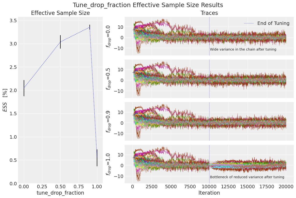
我们可以看到,当drop_tune_fraction等于0.5或0.9时,ESS较高,相比0.0或1.0。从轨迹来看,我们发现当drop_tune_fraction = 0.0时,调优后的链的方差较大。在另一个极端,当drop_tune_fraction = 1.0时,链通过了一个低方差的瓶颈。
自相关#
我们可以在上面的采样阶段看到效果的诊断指标是自相关性。自相关性越低越好。
plot_autocorr_drop_tune_fraction(df_results)
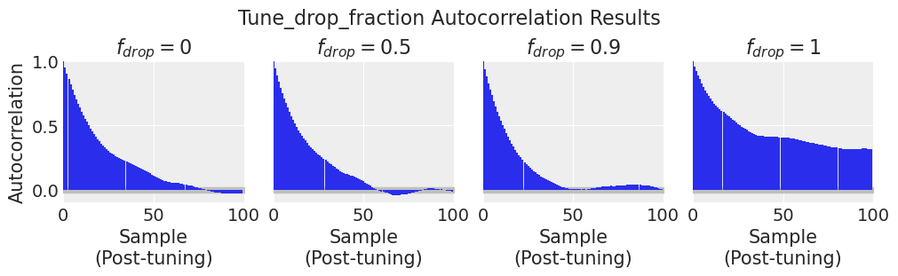
到第100步时,drop_tune_fraction = 0.9 的自相关性已经接近零。其他 drop_tune_fractions 的自相关性仍然较高,要么是因为采样步长太大(drop_tune_fraction = 0.0),要么是因为步长太小(drop_tune_fraction = 1.0)。当整个调优历史被丢弃时(drop_tune_fraction = 1.0),链必须从当前位置发散回典型集,这需要更长的时间。
接受率#
在 'accepted' 采样器统计数据上的滚动平均值显示了不同 drop_tune_fractions 下采样器性能的差异。调优后接受率的下降趋势表明提议开始时过于狭窄,而调优后接受率的上升趋势表明提议开始时过于宽泛。
plot_acceptance_rate_drop_tune_fraction(df_results)
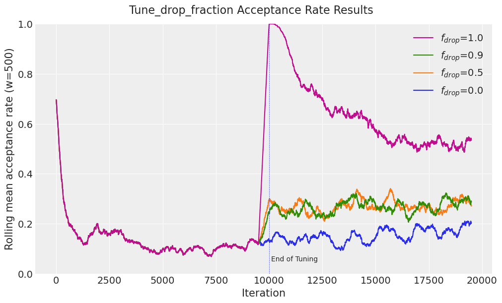
对于 drop_tune_fraction = 0.9 的接受率趋势大致持平。当调整历史被丢弃时(drop_tune_fraction = 1.0),接受率飙升至几乎 100%,因为提议过于狭窄。
总结#
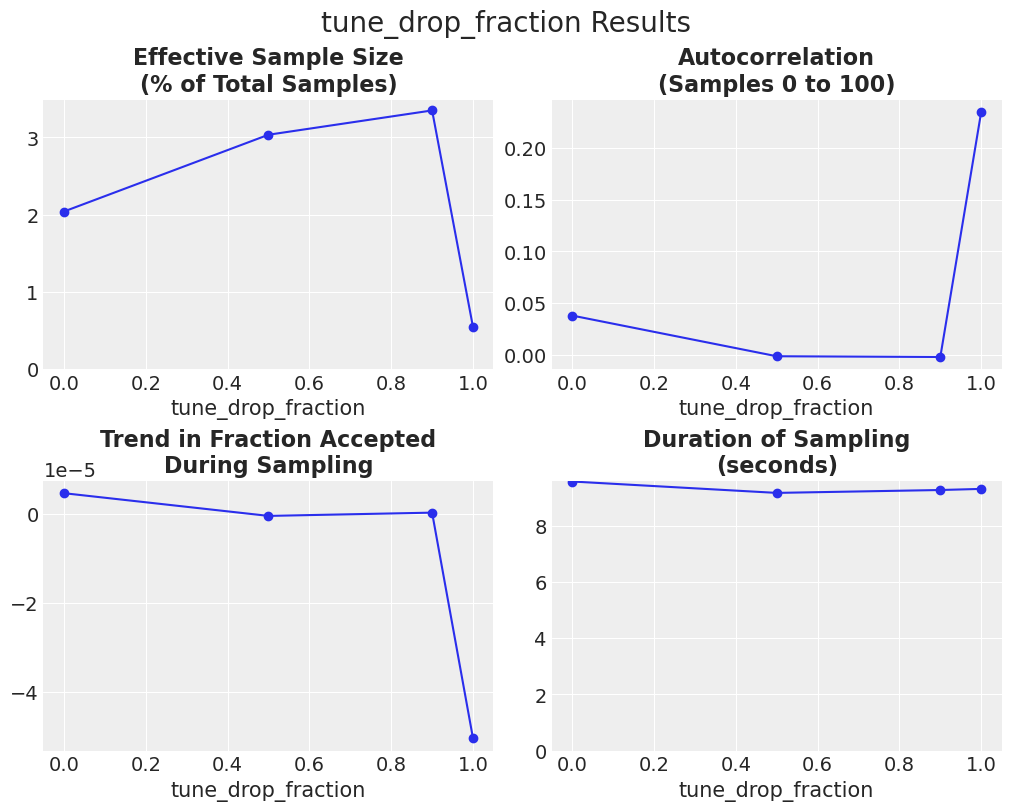
所有三个指标的结果以及采样持续时间如下所示。
plot_metric_results(df_results);
Lamb#
Lamb 是决定跳跃相对于随机向量大小的因子,并且默认情况下会进行调整。起始值为 \({2.38}/{\sqrt{2d}}\) 其中 \(d=\) 维数 [即参数]。我们将 lamb 在默认值上下一个数量级范围内变化,并调整 scaling 参数以保持 lamb 固定。
array([0.16829141, 0.37631104, 0.53218418, 0.75262208, 1.68291414])
df_results = sample_model_calc_metrics(
    model,
    param=param,
    param_values=lambs,
    step_kwargs=dict(tune="scaling"),
    N_tune=N_tune,
    N_draws=N_draws,
)
Show code cell output
plot_metric_results(df_results, param=param);
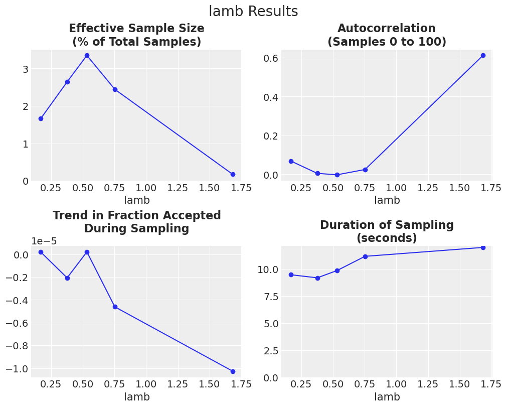
结果显示,lamb 的默认起始值(约为 0.5)是合适的。另请注意,这些结果可以与上述 drop_tune_fraction = 0.9 的结果进行比较,其中 lamb 被调整,并且 scaling 被指定为 0.001(默认值)。该调整设置的 ESS % 约为 1.8。因此,这些结果表明,在此问题中,固定 lamb 并调整 scaling 比固定 scaling 并调整 lamb 更好。
事后看来,这个结果是有道理的,因为随机向量项(lamb * \((x_{R1}-x_{R2})\))在采样过程中本质上是被缩放的,因为它是从之前的样本中抽取的。噪声项 \(\epsilon \sim \mathscr{D}_{p}(A)\)* scaling 在采样过程中是固定的,因此在采样之前调整 scaling 是有意义的。
缩放#
scaling 决定了噪声项的方差,默认值为0.001。我们将 scaling 的总变化范围设定为6个数量级,并调整 lamb。
scalings = np.array([1, 0.1, 0.01, 0.001, 0.0001, 0.00001])
param = "scaling"
df_results = sample_model_calc_metrics(
    model,
    param="scaling",
    param_values=scalings,
    step_kwargs=dict(tune="lambda"),
    N_tune=N_tune,
    N_draws=N_draws,
)
Show code cell output
axes = plot_metric_results(df_results, param=param)
for ax in axes.flatten():
    ax.set_xscale("log")
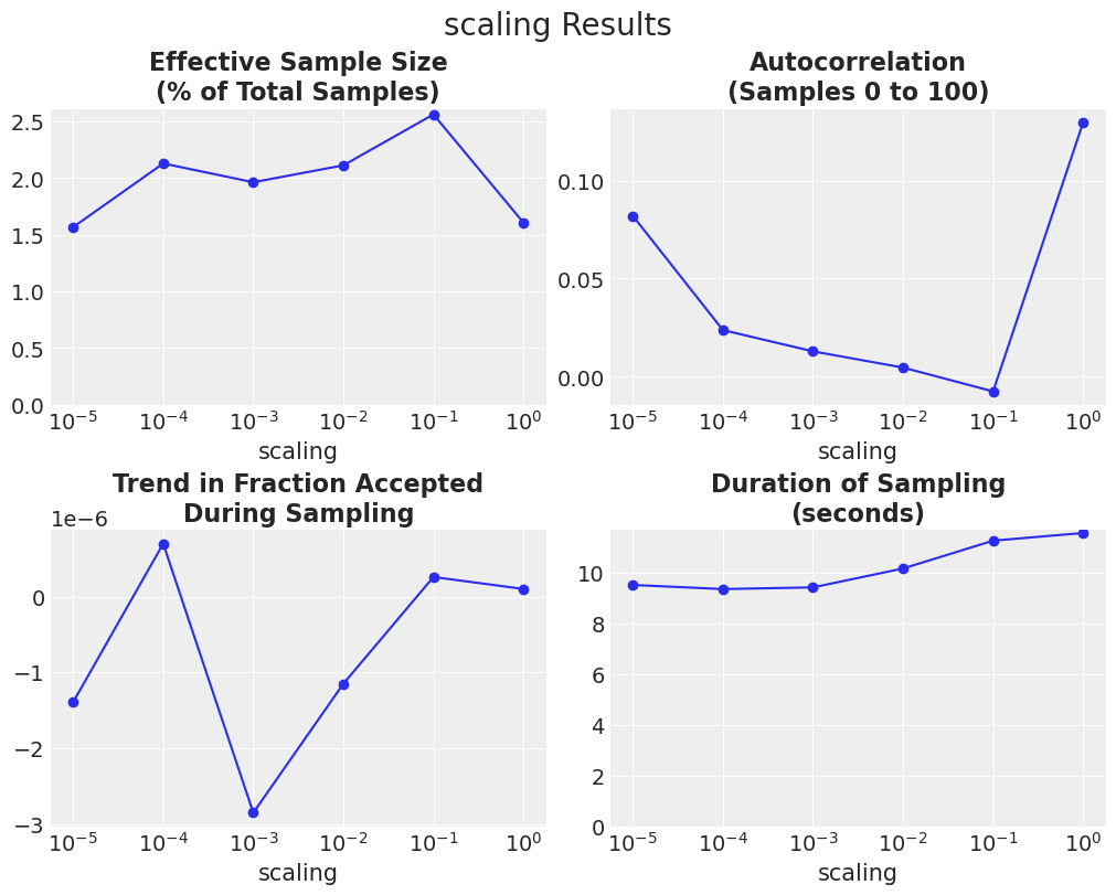
对于这个问题,较大的lamb值表现更好。 然而,调整scaling并固定lamb(之前的实验)表现更好。
提议分布#
最后,我们还可以改变proposal_distribution(\(\mathscr{D}_{p}\)),它决定了从哪个形状中抽取\(\epsilon\)。PyMC提供了四种用于连续变量的建议分布:均匀分布(默认)、正态分布、柯西分布和拉普拉斯分布。在这个实验中,我们将调整scaling,以允许每个建议分布进行优化,并保持lamb固定。
param = "proposal_dist"
proposal_dists = [pm.UniformProposal, pm.NormalProposal, pm.CauchyProposal, pm.LaplaceProposal]
df_results = sample_model_calc_metrics(
    model,
    param=param,
    param_values=proposal_dists,
    step_kwargs=dict(tune="scaling"),
    N_tune=N_tune,
    N_draws=N_draws,
)
Show code cell output
axes = plot_metric_results(df_results, param=param)
for ax in axes.flatten():
    labels = ax.get_xticklabels()
    ax.set_xticklabels(labels, rotation=45)
C:\Users\greg\AppData\Local\Temp\ipykernel_16780\1850776206.py:4: UserWarning: FixedFormatter should only be used together with FixedLocator
  ax.set_xticklabels(labels, rotation=45)
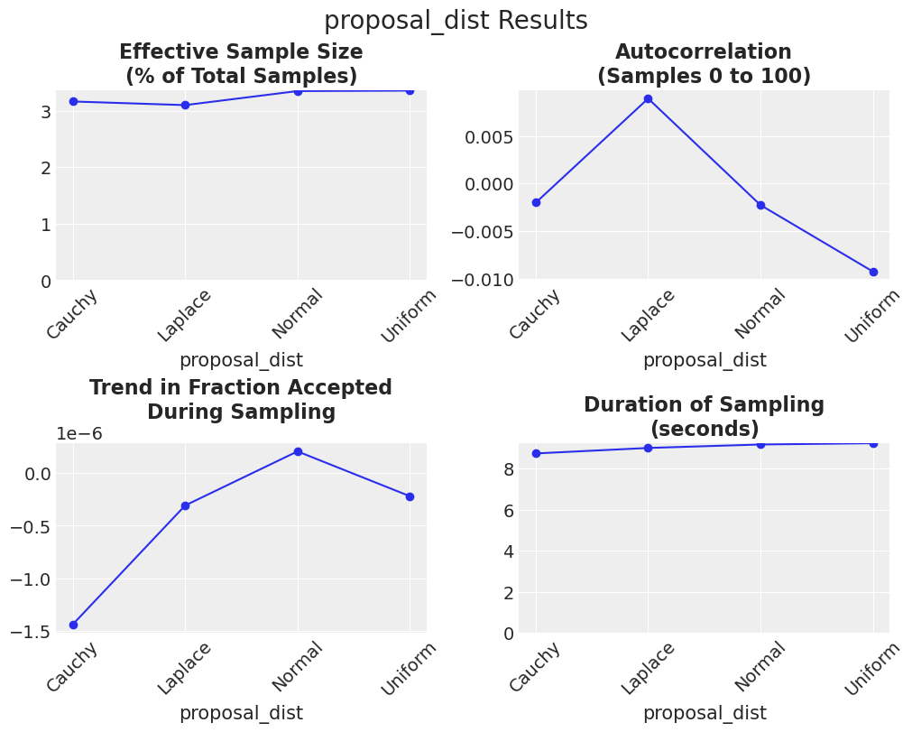
所有分布的表现都相当不错。考虑到所有三个指标,正态分布和均匀分布似乎比其他分布表现得稍好一些。请注意,ter Braak 和 Vrugt [2008] 建议 proposal_dist 应具有无界支持以保持遍历性,因此首选正态分布。
结论#
基于上述实验,针对此分布表现最佳的采样方案对默认设置进行了两项修改。以下是其简化形式:
with model:
    step = pm.DEMetropolisZ(tune="scaling", proposal_dist=pm.NormalProposal)
    idata = pm.sample(step=step, chains=1, tune=N_tune, draws=N_draws)
Sequential sampling (1 chains in 1 job)
DEMetropolisZ: [x]
Sampling 1 chain for 10_000 tune and 10_000 draw iterations (10_000 + 10_000 draws total) took 10 seconds.
Only one chain was sampled, this makes it impossible to run some convergence checks
print("ESS % =", calc_ess_pct(idata).mean().round(1))
ESS % = 2.9
参考资料#
Cajo J.F. ter Braak 和 Jasper A. Vrugt。带有 Snooker 更新器和更少链的差分进化马尔可夫链。统计与计算,第 435–446 页,2008 年。URL: https://link.springer.com/content/pdf/10.1007/s11222-008-9104-9.pdf?pdf=button。
%watermark -n -u -v -iv -w
Last updated: Fri Feb 10 2023

Python implementation: CPython
Python version       : 3.11.0
IPython version      : 8.7.0

arviz     : 0.14.0
sys       : 3.11.0 | packaged by conda-forge | (main, Oct 25 2022, 06:12:32) [MSC v.1929 64 bit (AMD64)]
numpy     : 1.24.0
pandas    : 1.5.2
matplotlib: 3.6.2
pymc      : 5.0.1+5.ga7f361bd

Watermark: 2.3.1