PyMC中\(AR(1)\)模型的分析#
import arviz as az
import matplotlib.pyplot as plt
import numpy as np
import pymc as pm
%config InlineBackend.figure_format = 'retina'
RANDOM_SEED = 8927
np.random.seed(RANDOM_SEED)
az.style.use("arviz-darkgrid")
考虑以下在无限过去初始化的AR(2)过程:
\[
y_t = \rho_0 + \rho_1 y_{t-1} + \rho_2 y_{t-2} + \epsilon_t,
\]
其中 \(\epsilon_t \overset{iid}{\sim} {\cal N}(0,1)\)。 假设您想从观测样本 \(Y^T = \{ y_0, y_1,\ldots, y_T \}\) 中了解 \(\rho\)。
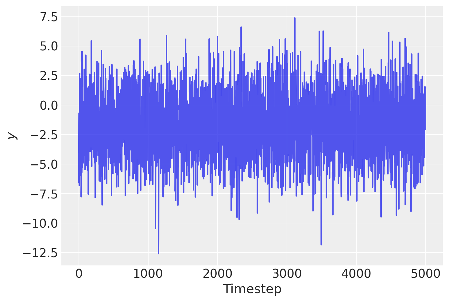
首先,让我们生成一些合成样本数据。我们通过从一个AR(2)过程中生成10,000个样本,然后丢弃前5,000个样本来模拟“无限过去”:
T = 10000

# true stationarity:
true_rho = 0.7, -0.3
# true standard deviation of the innovation:
true_sigma = 2.0
# true process mean:
true_center = -1.0

y = np.random.normal(loc=true_center, scale=true_sigma, size=T)
y[1] += true_rho[0] * y[0]
for t in range(2, T - 100):
    y[t] += true_rho[0] * y[t - 1] + true_rho[1] * y[t - 2]

y = y[-5000:]
plt.plot(y, alpha=0.8)
plt.xlabel("Timestep")
plt.ylabel("$y$");
让我们从尝试拟合错误的模型开始!假设我们不知道生成模型,因此为了简单起见,我们简单地拟合一个AR(1)模型。
这个生成过程在PyMC中实现起来相当直接。由于我们希望在AR过程中包含一个截距项,我们必须设置constant=True,否则当rho的大小为2时,PyMC会假设我们想要一个AR2过程。此外,默认情况下,初始值的先验分布将使用\(N(0, 100)\)。我们可以通过将一个分布(不是一个完整的随机变量)传递给init_dist参数来覆盖这个默认设置。
with pm.Model() as ar1:
    # assumes 95% of prob mass is between -2 and 2
    rho = pm.Normal("rho", mu=0.0, sigma=1.0, shape=2)
    # precision of the innovation term
    tau = pm.Exponential("tau", lam=0.5)

    likelihood = pm.AR(
        "y", rho=rho, tau=tau, constant=True, init_dist=pm.Normal.dist(0, 10), observed=y
    )

    idata = pm.sample(1000, tune=2000, random_seed=RANDOM_SEED)
Auto-assigning NUTS sampler...
Initializing NUTS using jitter+adapt_diag...
Multiprocess sampling (4 chains in 4 jobs)
NUTS: [rho, tau]
100.00% [12000/12000 00:04<00:00 Sampling 4 chains, 0 divergences]
Sampling 4 chains for 2_000 tune and 1_000 draw iterations (8_000 + 4_000 draws total) took 5 seconds.
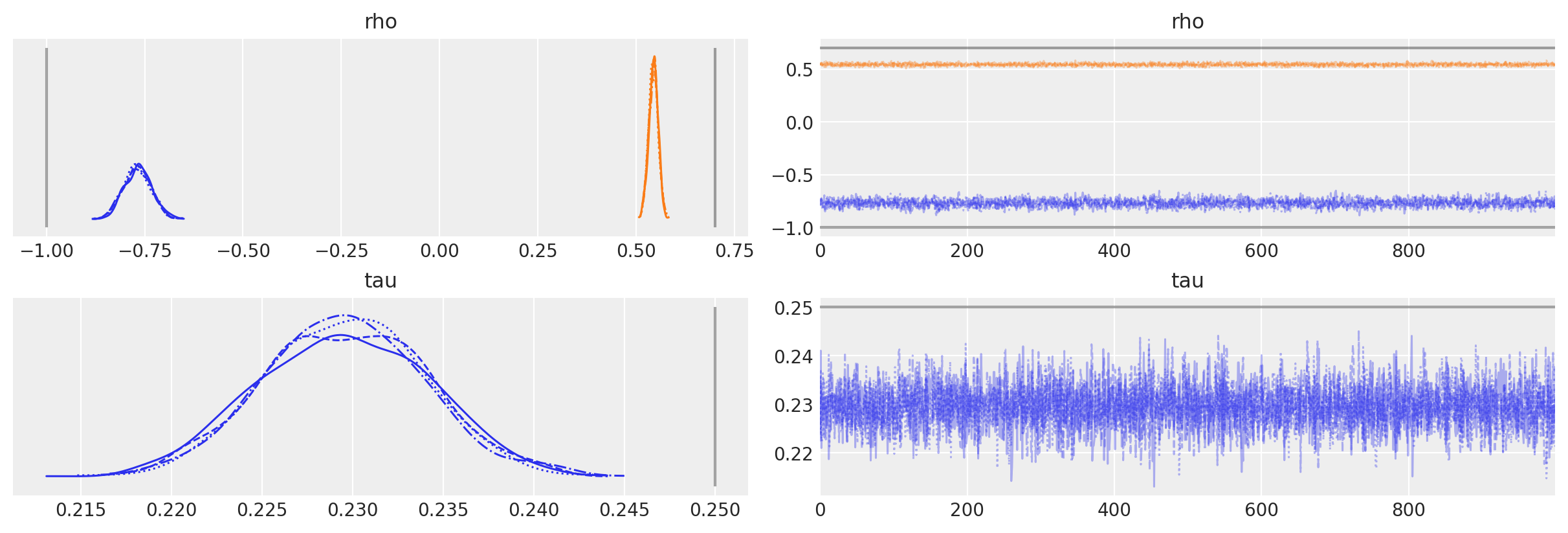
我们可以看到,尽管我们假设了错误的模型,参数估计值实际上与真实值相差并不远。
az.plot_trace(
    idata,
    lines=[
        ("rho", {}, [true_center, true_rho[0]]),
        ("tau", {}, true_sigma**-2),
    ],
);
扩展到AR(p)#
现在让我们拟合正确的潜在模型,一个AR(2):
\[
y_t = \rho_0 + \rho_1 y_{t-1} + \rho_2 y_{t-2} + \epsilon_t.
\]
AR分布通过传递给AR的rho参数的大小推断过程的顺序(包括均值)。
我们还将使用创新的标准差(而不是精度)来参数化分布。
with pm.Model() as ar2:
    rho = pm.Normal("rho", 0.0, 1.0, shape=3)
    sigma = pm.HalfNormal("sigma", 3)
    likelihood = pm.AR(
        "y", rho=rho, sigma=sigma, constant=True, init_dist=pm.Normal.dist(0, 10), observed=y
    )

    idata = pm.sample(
        1000,
        tune=2000,
        random_seed=RANDOM_SEED,
    )
Auto-assigning NUTS sampler...
Initializing NUTS using jitter+adapt_diag...
Multiprocess sampling (4 chains in 4 jobs)
NUTS: [rho, sigma]
100.00% [12000/12000 00:09<00:00 Sampling 4 chains, 0 divergences]
Sampling 4 chains for 2_000 tune and 1_000 draw iterations (8_000 + 4_000 draws total) took 9 seconds.
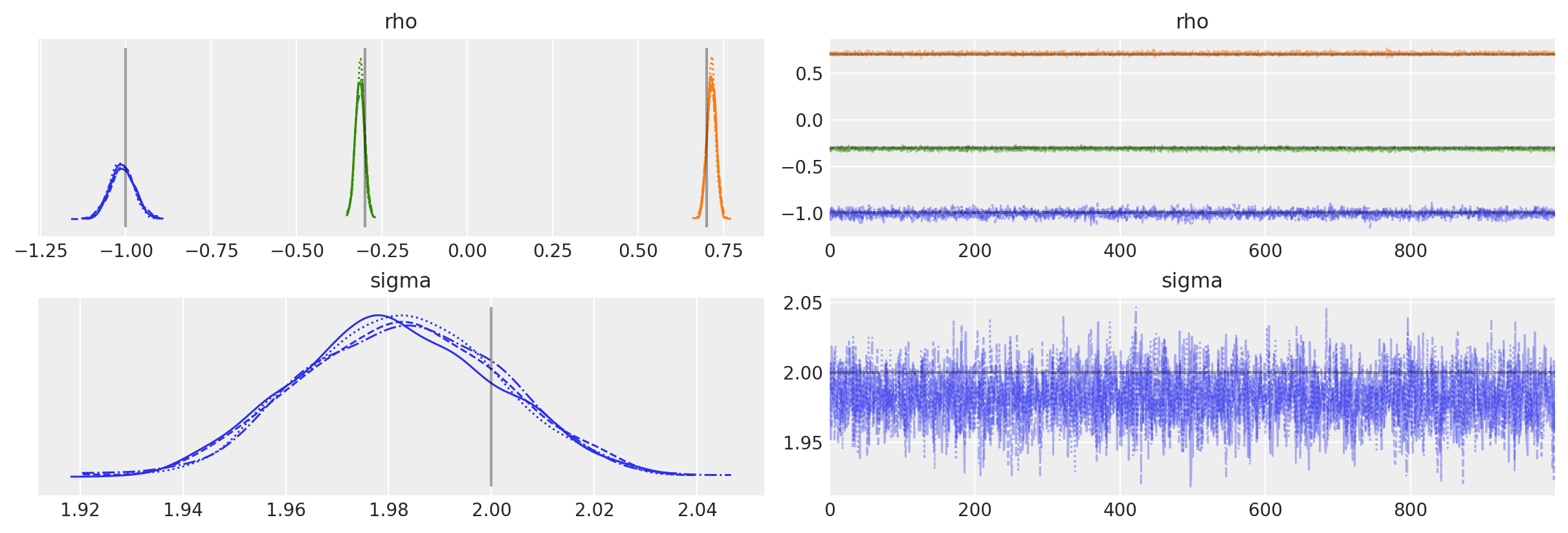
后验图显示我们已经正确推断出生成模型参数。
az.plot_trace(
    idata,
    lines=[
        ("rho", {}, (true_center,) + true_rho),
        ("sigma", {}, true_sigma),
    ],
);
如果AR参数不是同分布的,您也可以将它们作为列表传递。
import pytensor.tensor as pt

with pm.Model() as ar2_bis:
    rho0 = pm.Normal("rho0", mu=0.0, sigma=5.0)
    rho1 = pm.Uniform("rho1", -1, 1)
    rho2 = pm.Uniform("rho2", -1, 1)
    sigma = pm.HalfNormal("sigma", 3)
    likelihood = pm.AR(
        "y",
        rho=pt.stack([rho0, rho1, rho2]),
        sigma=sigma,
        constant=True,
        init_dist=pm.Normal.dist(0, 10),
        observed=y,
    )

    idata = pm.sample(
        1000,
        tune=2000,
        target_accept=0.9,
        random_seed=RANDOM_SEED,
    )
Auto-assigning NUTS sampler...
Initializing NUTS using jitter+adapt_diag...
Multiprocess sampling (4 chains in 4 jobs)
NUTS: [rho0, rho1, rho2, sigma]
100.00% [12000/12000 00:09<00:00 Sampling 4 chains, 0 divergences]
Sampling 4 chains for 2_000 tune and 1_000 draw iterations (8_000 + 4_000 draws total) took 10 seconds.
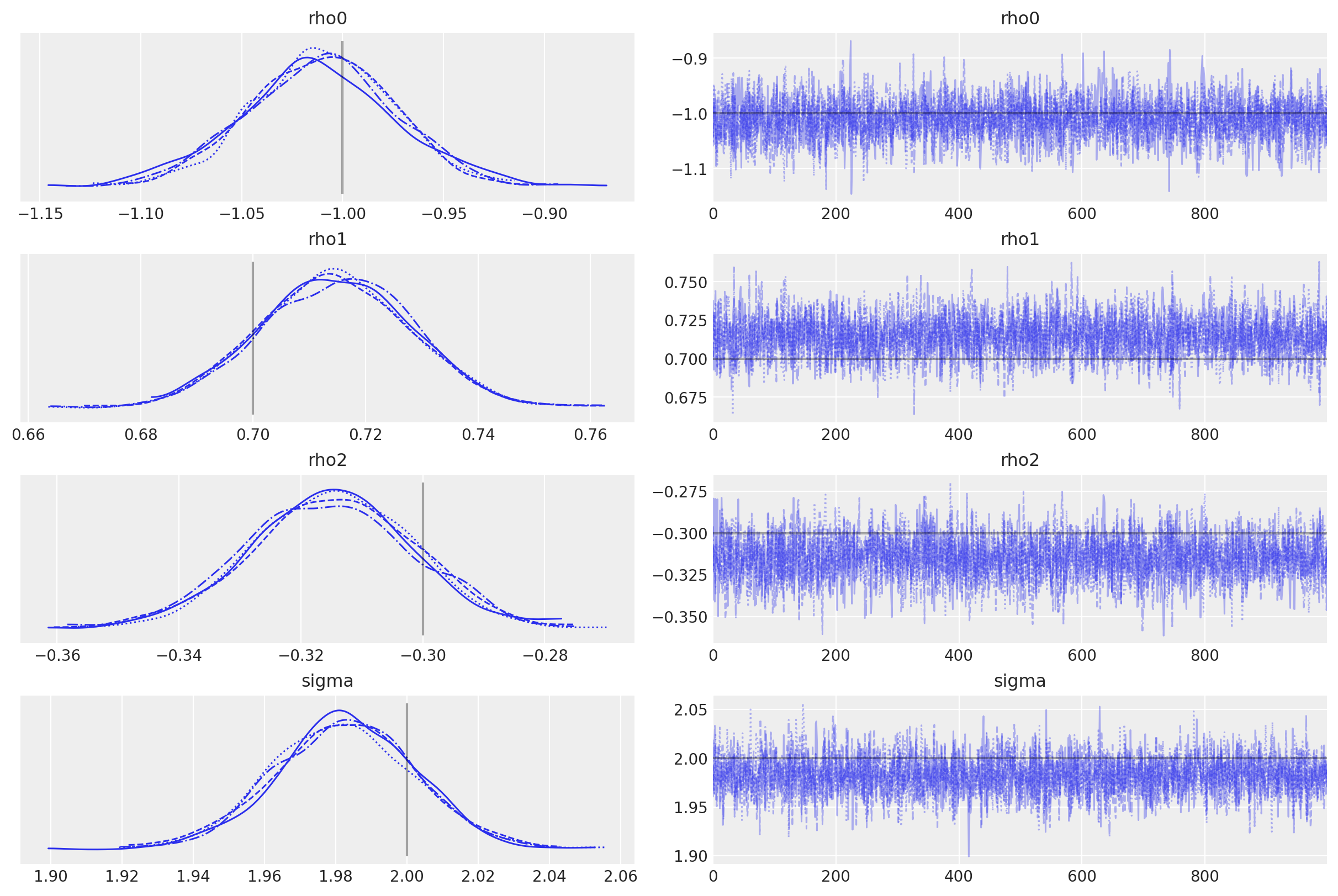
az.plot_trace(
    idata,
    lines=[
        ("rho0", {}, true_center),
        ("rho1", {}, true_rho[0]),
        ("rho2", {}, true_rho[1]),
        ("sigma", {}, true_sigma),
    ],
);