


航空乘客 - 类似Prophet的模型#
我们将研究“航空乘客”数据集,该数据集记录了1949年至1960年间美国航空公司每月乘客总数。我们可以使用Prophet模型来拟合这个数据集[Taylor 和 Letham, 2018](事实上,这个数据集是他们文档中的示例之一),但我们将在PyMC3中构建自己的类似Prophet的模型。这将使我们更容易检查模型的组件并进行先验预测检查(这是贝叶斯工作流程的一个组成部分[Gelman 等人, 2020])。
import arviz as az
import matplotlib.dates as mdates
import matplotlib.pyplot as plt
import numpy as np
import pandas as pd
import pymc as pm
RANDOM_SEED = 8927
rng = np.random.default_rng(RANDOM_SEED)
az.style.use("arviz-darkgrid")
%config InlineBackend.figure_format = 'retina'
# get data
try:
    df = pd.read_csv("../data/AirPassengers.csv", parse_dates=["Month"])
except FileNotFoundError:
    df = pd.read_csv(pm.get_data("AirPassengers.csv"), parse_dates=["Month"])
在我们开始之前:可视化数据#
df.plot.scatter(x="Month", y="#Passengers", color="k");
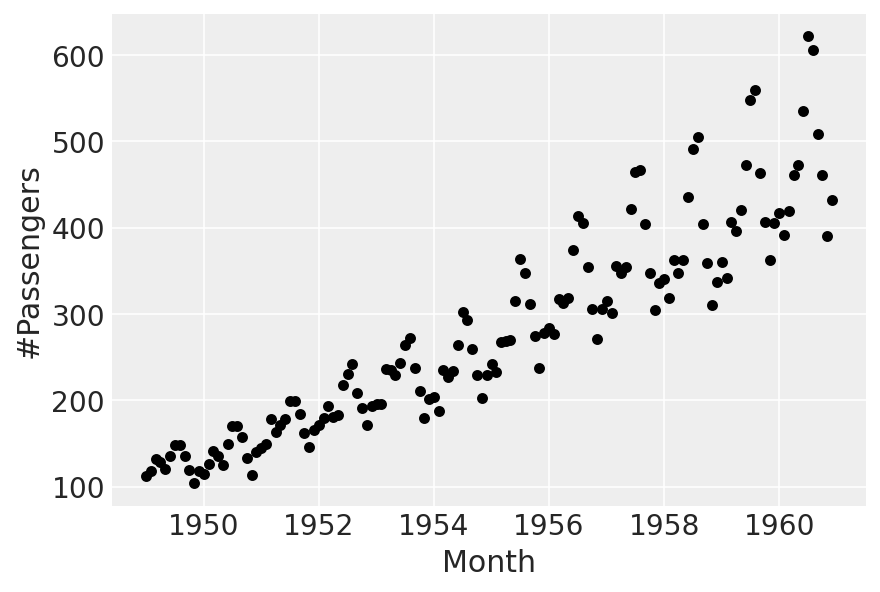
存在一个上升趋势,具有乘法季节性。我们将拟合一个线性趋势,并从Prophet中“借用”其乘法季节性部分。
第0部分:缩放数据#
首先,我们将时间缩放到0到1之间:
t = (df["Month"] - pd.Timestamp("1900-01-01")).dt.days.to_numpy()
t_min = np.min(t)
t_max = np.max(t)
t = (t - t_min) / (t_max - t_min)
接下来,对于目标变量,我们将其除以最大值。我们这样做,而不是标准化,以保持观测值的符号不变 - 这对于季节性成分在后续工作中正常运行是必要的。
y = df["#Passengers"].to_numpy()
y_max = np.max(y)
y = y / y_max
第一部分:线性趋势#
我们目前要拟合的模型将是
首先,让我们尝试使用prophet设定的默认先验,并进行先验预测检查:
with pm.Model(check_bounds=False) as linear:
    α = pm.Normal("α", mu=0, sigma=5)
    β = pm.Normal("β", mu=0, sigma=5)
    σ = pm.HalfNormal("σ", sigma=5)
    trend = pm.Deterministic("trend", α + β * t)
    pm.Normal("likelihood", mu=trend, sigma=σ, observed=y)

    linear_prior = pm.sample_prior_predictive()

fig, ax = plt.subplots(nrows=2, ncols=1, sharex=True)
ax[0].plot(
    df["Month"],
    az.extract_dataset(linear_prior, group="prior_predictive", num_samples=100)["likelihood"]
    * y_max,
    color="blue",
    alpha=0.05,
)
df.plot.scatter(x="Month", y="#Passengers", color="k", ax=ax[0])
ax[0].set_title("Prior predictive")
ax[1].plot(
    df["Month"],
    az.extract_dataset(linear_prior, group="prior", num_samples=100)["trend"] * y_max,
    color="blue",
    alpha=0.05,
)
df.plot.scatter(x="Month", y="#Passengers", color="k", ax=ax[1])
ax[1].set_title("Prior trend lines");
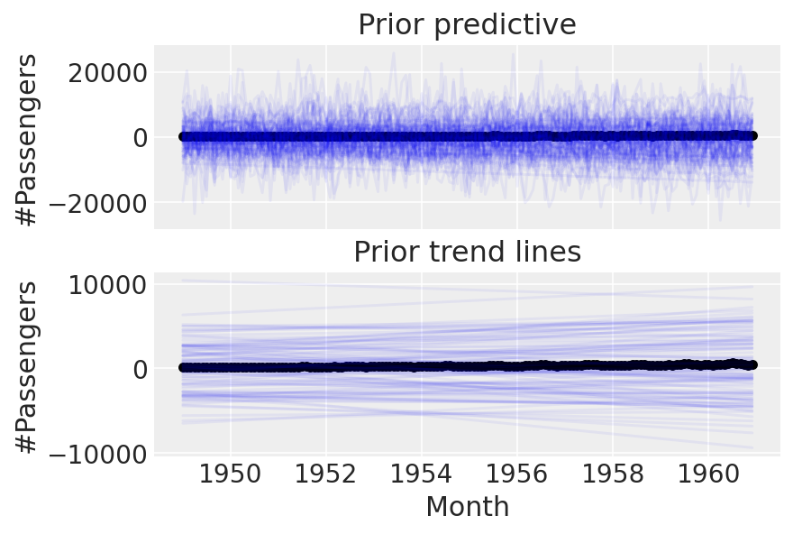
我们可以做得更好。这些先验显然太宽了,因为我们最终得到了难以置信的乘客数量。让我们尝试设置更严格的先验。
with pm.Model(check_bounds=False) as linear:
    α = pm.Normal("α", mu=0, sigma=0.5)
    β = pm.Normal("β", mu=0, sigma=0.5)
    σ = pm.HalfNormal("σ", sigma=0.1)
    trend = pm.Deterministic("trend", α + β * t)
    pm.Normal("likelihood", mu=trend, sigma=σ, observed=y)

    linear_prior = pm.sample_prior_predictive(samples=100)

fig, ax = plt.subplots(nrows=2, ncols=1, sharex=True)
ax[0].plot(
    df["Month"],
    az.extract_dataset(linear_prior, group="prior_predictive", num_samples=100)["likelihood"]
    * y_max,
    color="blue",
    alpha=0.05,
)
df.plot.scatter(x="Month", y="#Passengers", color="k", ax=ax[0])
ax[0].set_title("Prior predictive")
ax[1].plot(
    df["Month"],
    az.extract_dataset(linear_prior, group="prior", num_samples=100)["trend"] * y_max,
    color="blue",
    alpha=0.05,
)
df.plot.scatter(x="Month", y="#Passengers", color="k", ax=ax[1])
ax[1].set_title("Prior trend lines");
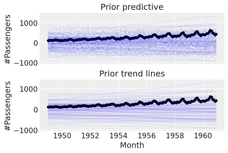
好的。在进入更复杂的内容之前,让我们先尝试对数据进行条件处理并进行后验预测检查:
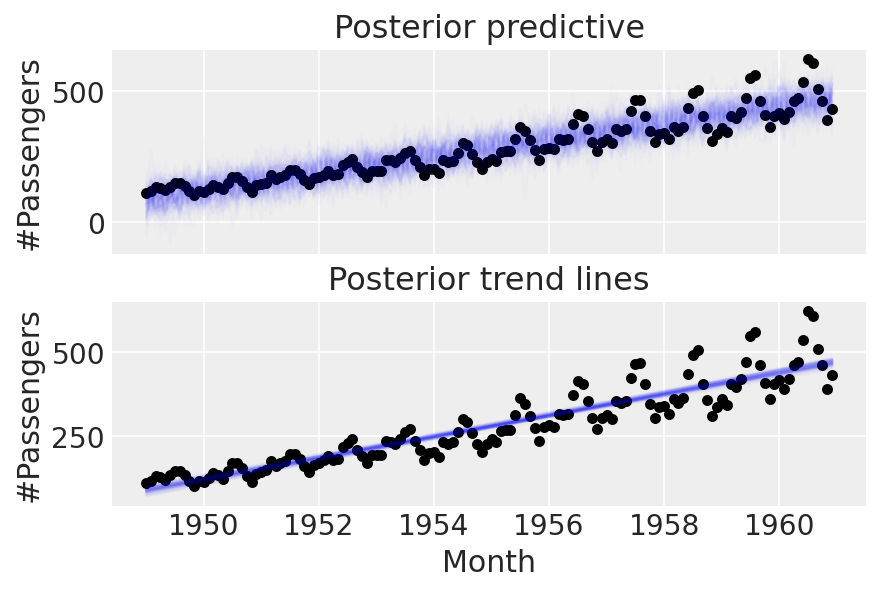
with linear:
    linear_trace = pm.sample(return_inferencedata=True)
    linear_prior = pm.sample_posterior_predictive(trace=linear_trace)

fig, ax = plt.subplots(nrows=2, ncols=1, sharex=True)
ax[0].plot(
    df["Month"],
    az.extract_dataset(linear_prior, group="posterior_predictive", num_samples=100)["likelihood"]
    * y_max,
    color="blue",
    alpha=0.01,
)
df.plot.scatter(x="Month", y="#Passengers", color="k", ax=ax[0])
ax[0].set_title("Posterior predictive")
ax[1].plot(
    df["Month"],
    az.extract_dataset(linear_trace, group="posterior", num_samples=100)["trend"] * y_max,
    color="blue",
    alpha=0.01,
)
df.plot.scatter(x="Month", y="#Passengers", color="k", ax=ax[1])
ax[1].set_title("Posterior trend lines");
Auto-assigning NUTS sampler...
Initializing NUTS using jitter+adapt_diag...
Multiprocess sampling (4 chains in 4 jobs)
NUTS: [α, β, σ]
Sampling 4 chains for 1_000 tune and 1_000 draw iterations (4_000 + 4_000 draws total) took 3 seconds.
The acceptance probability does not match the target. It is 0.8849, but should be close to 0.8. Try to increase the number of tuning steps.
The acceptance probability does not match the target. It is 0.8801, but should be close to 0.8. Try to increase the number of tuning steps.
第二部分:输入季节性#
为了建模季节性,我们将“借用”Prophet采用的方法 - 详情请参见Prophet论文 [Taylor 和 Letham, 2018],但基本思想是制作一个傅里叶特征矩阵,该矩阵与系数向量相乘。由于我们将使用乘法季节性,最终模型将是
n_order = 10
periods = (df["Month"] - pd.Timestamp("1900-01-01")).dt.days / 365.25

fourier_features = pd.DataFrame(
    {
        f"{func}_order_{order}": getattr(np, func)(2 * np.pi * periods * order)
        for order in range(1, n_order + 1)
        for func in ("sin", "cos")
    }
)
fourier_features
| sin_order_1 | cos_order_1 | sin_order_2 | cos_order_2 | sin_order_3 | cos_order_3 | sin_order_4 | cos_order_4 | sin_order_5 | cos_order_5 | sin_order_6 | cos_order_6 | sin_order_7 | cos_order_7 | sin_order_8 | cos_order_8 | sin_order_9 | cos_order_9 | sin_order_10 | cos_order_10 | |
|---|---|---|---|---|---|---|---|---|---|---|---|---|---|---|---|---|---|---|---|---|
| 0 | -0.004301 | 0.999991 | -0.008601 | 0.999963 | -0.012901 | 0.999917 | -0.017202 | 0.999852 | -0.021501 | 0.999769 | -0.025801 | 0.999667 | -0.030100 | 0.999547 | -0.034398 | 0.999408 | -0.038696 | 0.999251 | -0.042993 | 0.999075 |
| 1 | 0.504648 | 0.863325 | 0.871351 | 0.490660 | 0.999870 | -0.016127 | 0.855075 | -0.518505 | 0.476544 | -0.879150 | -0.032249 | -0.999480 | -0.532227 | -0.846602 | -0.886721 | -0.462305 | -0.998830 | 0.048363 | -0.837909 | 0.545811 |
| 2 | 0.847173 | 0.531317 | 0.900235 | -0.435405 | 0.109446 | -0.993993 | -0.783934 | -0.620844 | -0.942480 | 0.334263 | -0.217577 | 0.976043 | 0.711276 | 0.702913 | 0.973402 | -0.229104 | 0.323093 | -0.946367 | -0.630072 | -0.776537 |
| 3 | 0.999639 | 0.026876 | 0.053732 | -0.998555 | -0.996751 | -0.080549 | -0.107308 | 0.994226 | 0.990983 | 0.133990 | 0.160575 | -0.987024 | -0.982352 | -0.187043 | -0.213377 | 0.976970 | 0.970882 | 0.239557 | 0.265563 | -0.964094 |
| 4 | 0.882712 | -0.469915 | -0.829598 | -0.558361 | -0.103031 | 0.994678 | 0.926430 | -0.376467 | -0.767655 | -0.640864 | -0.204966 | 0.978769 | 0.960288 | -0.279012 | -0.697540 | -0.716546 | -0.304719 | 0.952442 | 0.983924 | -0.178587 |
| ... | ... | ... | ... | ... | ... | ... | ... | ... | ... | ... | ... | ... | ... | ... | ... | ... | ... | ... | ... | ... |
| 139 | -0.484089 | -0.875019 | 0.847173 | 0.531317 | -0.998497 | -0.054805 | 0.900235 | -0.435405 | -0.576948 | 0.816781 | 0.109446 | -0.993993 | 0.385413 | 0.922744 | -0.783934 | -0.620844 | 0.986501 | 0.163757 | -0.942480 | 0.334263 |
| 140 | -0.861693 | -0.507430 | 0.874498 | -0.485029 | -0.025801 | 0.999667 | -0.848314 | -0.529494 | 0.886721 | -0.462305 | -0.051584 | 0.998669 | -0.834370 | -0.551205 | 0.898354 | -0.439273 | -0.077334 | 0.997005 | -0.819871 | -0.572548 |
| 141 | -0.999870 | -0.016127 | 0.032249 | -0.999480 | 0.998830 | 0.048363 | -0.064464 | 0.997920 | -0.996751 | -0.080549 | 0.096613 | -0.995322 | 0.993635 | 0.112651 | -0.128661 | 0.991689 | -0.989485 | -0.144636 | 0.160575 | -0.987024 |
| 142 | -0.869233 | 0.494403 | -0.859503 | -0.511131 | 0.019352 | -0.999813 | 0.878637 | -0.477489 | 0.849450 | 0.527668 | -0.038696 | 0.999251 | -0.887713 | 0.460397 | -0.839080 | -0.544008 | 0.058026 | -0.998315 | 0.896456 | -0.443132 |
| 143 | -0.512055 | 0.858953 | -0.879662 | 0.475599 | -0.999121 | -0.041919 | -0.836733 | -0.547611 | -0.438307 | -0.898825 | 0.083764 | -0.996486 | 0.582205 | -0.813042 | 0.916409 | -0.400244 | 0.992099 | 0.125461 | 0.787922 | 0.615774 |
144 行 × 20 列
再次,让我们使用默认的Prophet先验,只是为了看看会发生什么。
coords = {"fourier_features": np.arange(2 * n_order)}
with pm.Model(check_bounds=False, coords=coords) as linear_with_seasonality:
    α = pm.Normal("α", mu=0, sigma=0.5)
    β = pm.Normal("β", mu=0, sigma=0.5)
    σ = pm.HalfNormal("σ", sigma=0.1)
    β_fourier = pm.Normal("β_fourier", mu=0, sigma=10, dims="fourier_features")
    seasonality = pm.Deterministic(
        "seasonality", pm.math.dot(β_fourier, fourier_features.to_numpy().T)
    )
    trend = pm.Deterministic("trend", α + β * t)
    μ = trend * (1 + seasonality)
    pm.Normal("likelihood", mu=μ, sigma=σ, observed=y)

    linear_seasonality_prior = pm.sample_prior_predictive()

fig, ax = plt.subplots(nrows=3, ncols=1, sharex=False, figsize=(8, 6))
ax[0].plot(
    df["Month"],
    az.extract_dataset(linear_seasonality_prior, group="prior_predictive", num_samples=100)[
        "likelihood"
    ]
    * y_max,
    color="blue",
    alpha=0.05,
)
df.plot.scatter(x="Month", y="#Passengers", color="k", ax=ax[0])
ax[0].set_title("Prior predictive")
ax[1].plot(
    df["Month"],
    az.extract_dataset(linear_seasonality_prior, group="prior", num_samples=100)["trend"] * y_max,
    color="blue",
    alpha=0.05,
)
df.plot.scatter(x="Month", y="#Passengers", color="k", ax=ax[1])
ax[1].set_title("Prior trend lines")
ax[2].plot(
    df["Month"].iloc[:12],
    az.extract_dataset(linear_seasonality_prior, group="prior", num_samples=100)["seasonality"][:12]
    * 100,
    color="blue",
    alpha=0.05,
)
ax[2].set_title("Prior seasonality")
ax[2].set_ylabel("Percent change")
formatter = mdates.DateFormatter("%b")
ax[2].xaxis.set_major_formatter(formatter);
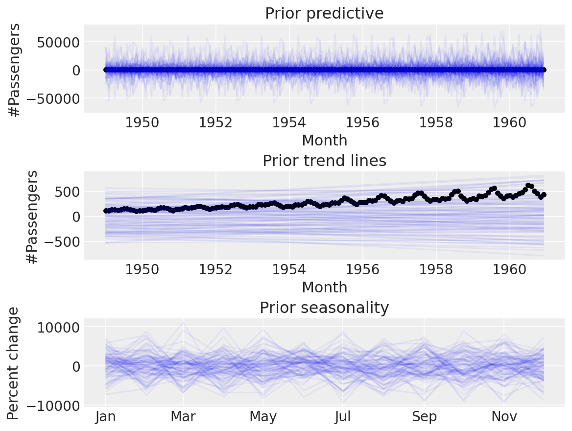
再次强调,这似乎不太合理。默认的先验分布对于我们的用例来说太宽了,而且在我们可以通过先验预测检查来设置更合理的先验分布时,使用它们是没有意义的。让我们尝试使用一些更窄的先验分布:
coords = {"fourier_features": np.arange(2 * n_order)}
with pm.Model(check_bounds=False, coords=coords) as linear_with_seasonality:
    α = pm.Normal("α", mu=0, sigma=0.5)
    β = pm.Normal("β", mu=0, sigma=0.5)
    trend = pm.Deterministic("trend", α + β * t)

    β_fourier = pm.Normal("β_fourier", mu=0, sigma=0.1, dims="fourier_features")
    seasonality = pm.Deterministic(
        "seasonality", pm.math.dot(β_fourier, fourier_features.to_numpy().T)
    )

    μ = trend * (1 + seasonality)
    σ = pm.HalfNormal("σ", sigma=0.1)
    pm.Normal("likelihood", mu=μ, sigma=σ, observed=y)

    linear_seasonality_prior = pm.sample_prior_predictive()

fig, ax = plt.subplots(nrows=3, ncols=1, sharex=False, figsize=(8, 6))
ax[0].plot(
    df["Month"],
    az.extract_dataset(linear_seasonality_prior, group="prior_predictive", num_samples=100)[
        "likelihood"
    ]
    * y_max,
    color="blue",
    alpha=0.05,
)
df.plot.scatter(x="Month", y="#Passengers", color="k", ax=ax[0])
ax[0].set_title("Prior predictive")
ax[1].plot(
    df["Month"],
    az.extract_dataset(linear_seasonality_prior, group="prior", num_samples=100)["trend"] * y_max,
    color="blue",
    alpha=0.05,
)
df.plot.scatter(x="Month", y="#Passengers", color="k", ax=ax[1])
ax[1].set_title("Prior trend lines")
ax[2].plot(
    df["Month"].iloc[:12],
    az.extract_dataset(linear_seasonality_prior, group="prior", num_samples=100)["seasonality"][:12]
    * 100,
    color="blue",
    alpha=0.05,
)
ax[2].set_title("Prior seasonality")
ax[2].set_ylabel("Percent change")
formatter = mdates.DateFormatter("%b")
ax[2].xaxis.set_major_formatter(formatter);
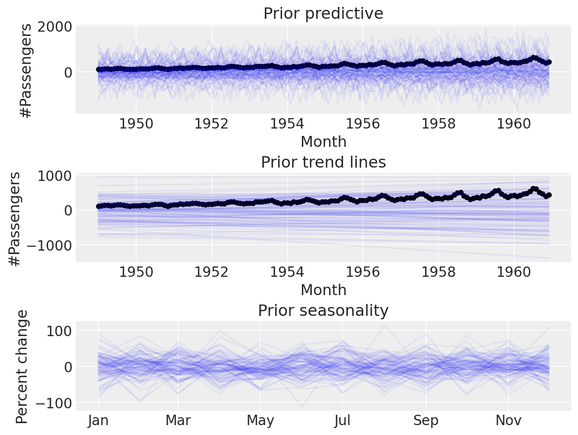
看起来更加可信了。现在是进行后验预测检查的时候了:
with linear_with_seasonality:
    linear_seasonality_trace = pm.sample(return_inferencedata=True)
    linear_seasonality_posterior = pm.sample_posterior_predictive(trace=linear_seasonality_trace)

fig, ax = plt.subplots(nrows=3, ncols=1, sharex=False, figsize=(8, 6))
ax[0].plot(
    df["Month"],
    az.extract_dataset(linear_seasonality_posterior, group="posterior_predictive", num_samples=100)[
        "likelihood"
    ]
    * y_max,
    color="blue",
    alpha=0.05,
)
df.plot.scatter(x="Month", y="#Passengers", color="k", ax=ax[0])
ax[0].set_title("Posterior predictive")
ax[1].plot(
    df["Month"],
    az.extract_dataset(linear_trace, group="posterior", num_samples=100)["trend"] * y_max,
    color="blue",
    alpha=0.05,
)
df.plot.scatter(x="Month", y="#Passengers", color="k", ax=ax[1])
ax[1].set_title("Posterior trend lines")
ax[2].plot(
    df["Month"].iloc[:12],
    az.extract_dataset(linear_seasonality_trace, group="posterior", num_samples=100)["seasonality"][
        :12
    ]
    * 100,
    color="blue",
    alpha=0.05,
)
ax[2].set_title("Posterior seasonality")
ax[2].set_ylabel("Percent change")
formatter = mdates.DateFormatter("%b")
ax[2].xaxis.set_major_formatter(formatter);
Auto-assigning NUTS sampler...
Initializing NUTS using jitter+adapt_diag...
Multiprocess sampling (4 chains in 4 jobs)
NUTS: [α, β, β_fourier, σ]
Sampling 4 chains for 1_000 tune and 1_000 draw iterations (4_000 + 4_000 draws total) took 16 seconds.
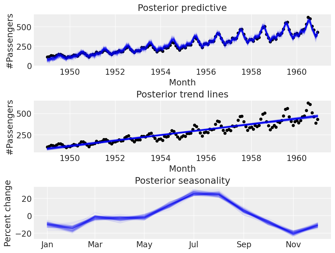
太棒了!
结论#
我们看到了如何自己实现一个类似Prophet的模型,并将其拟合到航空乘客数据集上。Prophet是一个非常棒的库,对社区来说是一个净积极因素,但通过自己实现它,我们可以选择我们认为与我们的问题相关的任何组件,对其进行定制,并执行贝叶斯工作流程[Gelman 等, 2020])。下次你遇到时间序列问题时,我希望你能尝试实现自己的概率模型,而不是将Prophet作为一个“黑箱”,其参数是可调的超参数。
作为参考,您可能还想要查看:
TimeSeeers,一个基于Facebook的Prophet的分层贝叶斯时间序列模型,使用PyMC3编写
PM-Prophet,一个基于Pymc3的通用时间序列预测和分解库,灵感来自Facebook Prophet
参考资料#
Sean J Taylor 和 Benjamin Letham。大规模预测。美国统计学家,72(1):37–45, 2018。URL: https://peerj.com/preprints/3190/。
安德鲁·格尔曼、阿基·维塔里、丹尼尔·辛普森、查尔斯·C·马戈西安、鲍勃·卡彭特、俞凌、劳伦·肯尼迪、乔纳·加布里、保罗-克里斯蒂安·比尔克纳、马丁·莫德拉克。贝叶斯工作流程。arXiv预印本arXiv:2011.01808,2020年。URL: https://arxiv.org/abs/2011.01808。
%load_ext watermark
%watermark -n -u -v -iv -w -p pytensor,aeppl,xarray
Last updated: Sun May 29 2022

Python implementation: CPython
Python version       : 3.9.12
IPython version      : 8.3.0

pytensor: 2.6.2
aeppl : 0.0.28
xarray: 2022.3.0

arviz     : 0.12.1
matplotlib: 3.5.2
pymc      : 4.0.0b6
numpy     : 1.22.4
pandas    : 1.4.2

Watermark: 2.3.0