


因子分析#
因子分析是一种广泛使用的概率模型,用于识别多元数据中的低秩结构,这些结构编码在潜在变量中。它与主成分分析非常密切相关,区别仅在于对这些潜在变量假设的先验分布。它也是一个线性高斯模型的良好示例,因为它可以完全描述为底层高斯变量的线性变换。有关因子分析与其他模型关系的概述,您可以查看此图,该图最初由Ghahramani和Roweis发表。
注意
本笔记本使用了不是 PyMC 依赖项的库,因此需要专门安装这些库才能运行此笔记本。打开下面的下拉菜单以获取更多指导。
Extra dependencies install instructions
为了在本地或binder上运行此笔记本,您不仅需要一个安装了所有可选依赖项的PyMC工作环境,还需要安装一些额外的依赖项。有关安装PyMC本身的建议,请参阅安装
您可以使用您喜欢的包管理器安装这些依赖项,我们提供了以下作为示例的pip和conda命令。
$ pip install seaborn
请注意,如果您想(或需要)从笔记本内部而不是命令行安装软件包,您可以通过运行pip命令的变体来安装软件包:
导入系统
!{sys.executable} -m pip install seaborn
您不应运行!pip install,因为它可能会在不同的环境中安装包,即使安装了也无法从Jupyter笔记本中使用。
另一个替代方案是使用conda:
$ conda install seaborn
在安装科学计算Python包时,我们推荐使用conda forge
import arviz as az
import numpy as np
import pymc as pm
import pytensor.tensor as pt
import scipy as sp
import seaborn as sns
import xarray as xr

from matplotlib import pyplot as plt
from matplotlib.lines import Line2D
from numpy.random import default_rng
from xarray_einstats import linalg
from xarray_einstats.stats import XrContinuousRV

print(f"Running on PyMC v{pm.__version__}")
Running on PyMC v5.10.2
%config InlineBackend.figure_format = 'retina'
az.style.use("arviz-darkgrid")

np.set_printoptions(precision=3, suppress=True)
RANDOM_SEED = 31415
rng = default_rng(RANDOM_SEED)
模拟数据生成#
为了通过几个示例进行操作,我们首先生成一些数据。这些数据不会遵循因子分析模型所假设的生成过程,因为潜在变量不会是高斯分布的。我们将假设我们有一个具有\(N\)行和\(d\)列的观测数据集,这些列实际上是\(k_{true}\)潜在变量的噪声线性函数。
n = 250
k_true = 4
d = 10
下一个代码单元通过创建潜在变量数组 M 和线性变换 Q 来生成数据。然后,矩阵乘积 \(QM\) 通过由方差参数 err_sd 控制的加性高斯噪声进行扰动。
由于我们生成数据的方式,表示\(Y\)列之间相关性的协方差矩阵将等于\(QQ^T\)。PCA和因子分析的基本假设是\(QQ^T\)不是满秩的。如果我们绘制协方差矩阵,我们可以看到这一点的暗示:
plt.figure(figsize=(4, 3))
sns.heatmap(np.corrcoef(Y));
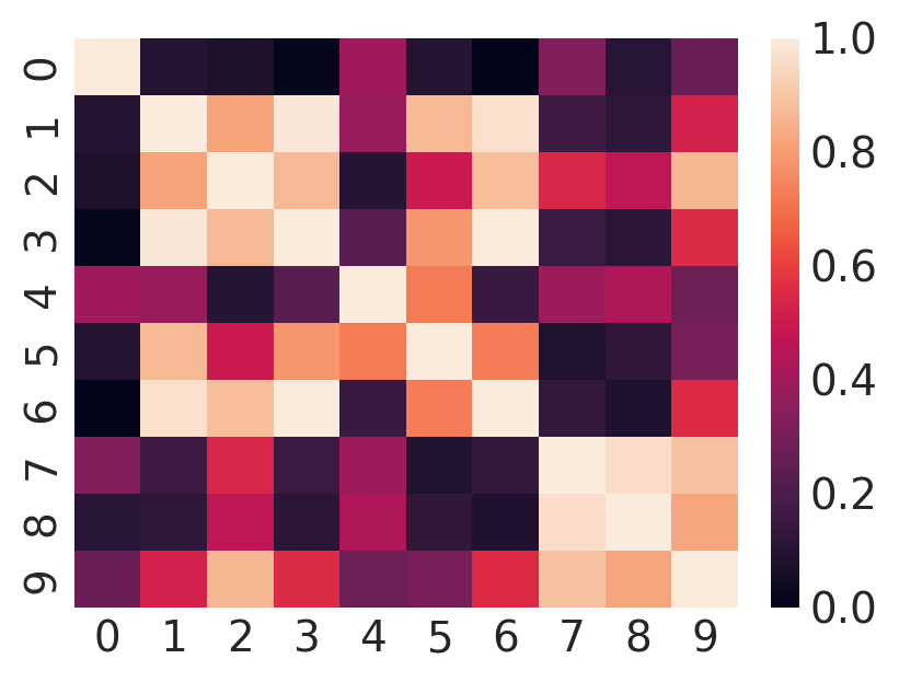
如果你眯着眼睛看足够久,你可能会发现一些地方,其中不同的列很可能是彼此的线性函数。
模型#
概率PCA(PPCA)和因子分析(FA)是PyMC论坛上常见的话题。下面链接的帖子处理了问题的不同方面,包括:
直接实现#
因子分析的模型是概率矩阵分解
\(X_{(d,n)}|W_{(d,k)}, F_{(k,n)} \sim \mathcal{N}(WF, \Psi)\)
其中 \(\Psi\) 是一个对角矩阵。下标表示矩阵的维度。概率PCA是一种变体,它设定 \(\Psi = \sigma^2 I\)。一个基本的实现(取自 这个gist)显示在下一个单元格中。不幸的是,它具有不适合模型拟合的不良特性。
k = 2

coords = {"latent_columns": np.arange(k), "rows": np.arange(n), "observed_columns": np.arange(d)}

with pm.Model(coords=coords) as PPCA:
    W = pm.Normal("W", dims=("observed_columns", "latent_columns"))
    F = pm.Normal("F", dims=("latent_columns", "rows"))
    sigma = pm.HalfNormal("sigma", 1.0)
    X = pm.Normal("X", mu=W @ F, sigma=sigma, observed=Y, dims=("observed_columns", "rows"))

    trace = pm.sample(tune=2000, random_seed=rng)  # target_accept=0.9
Auto-assigning NUTS sampler...
Initializing NUTS using jitter+adapt_diag...
Multiprocess sampling (4 chains in 4 jobs)
NUTS: [W, F, sigma]
Sampling 4 chains for 2_000 tune and 1_000 draw iterations (8_000 + 4_000 draws total) took 29 seconds.
The rhat statistic is larger than 1.01 for some parameters. This indicates problems during sampling. See https://arxiv.org/abs/1903.08008 for details
The effective sample size per chain is smaller than 100 for some parameters.  A higher number is needed for reliable rhat and ess computation. See https://arxiv.org/abs/1903.08008 for details
此时,已经出现了几个关于收敛检查失败的警告。我们可以在下面的轨迹图中看到更多问题。该图显示了每个采样器链在矩阵\(W\)中单个条目的路径,以及每个链的样本平均值。
for i in trace.posterior.chain.values:
    samples = trace.posterior["W"].sel(chain=i, observed_columns=3, latent_columns=1)
    plt.plot(samples, label="Chain {}".format(i + 1))
    plt.axhline(samples.mean(), color=f"C{i}")
plt.legend(ncol=4, loc="upper center", fontsize=12, frameon=True), plt.xlabel("Sample");
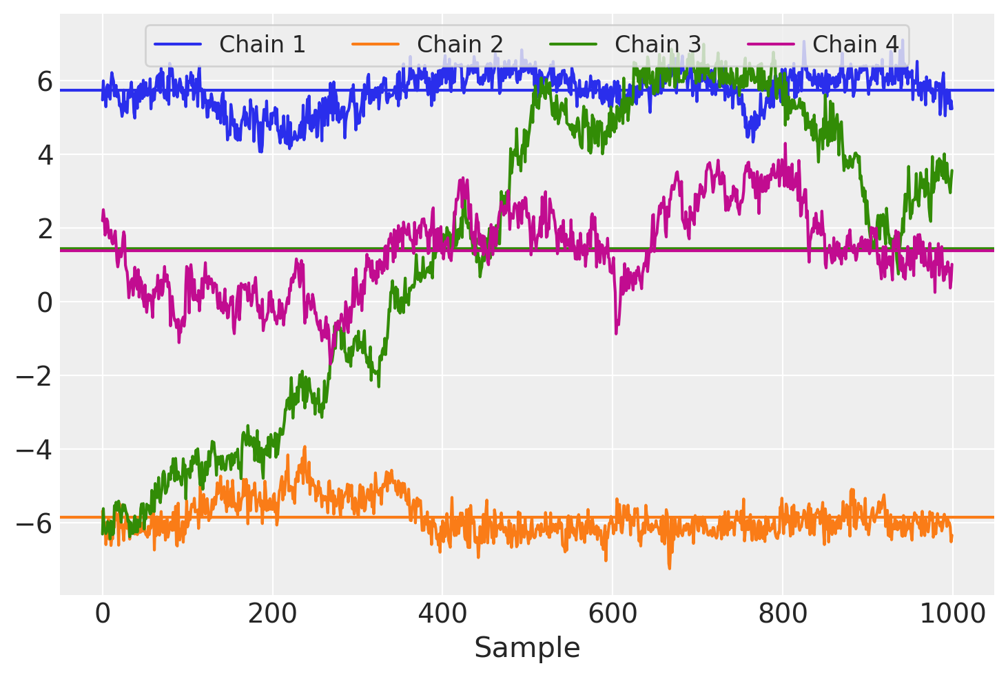
每个链似乎都有不同的样本均值,我们还可以看到链之间存在大量的自相关性,表现为采样迭代中的长期趋势。
该模型公式的主要缺点之一是其缺乏可识别性。在这种模型表示中,只有乘积 \(WF\) 对 \(X\) 的可能性有影响,因此对于任何可逆矩阵 \(\Omega\),有 \(P(X|W, F) = P(X|W\Omega, \Omega^{-1}F)\)。虽然 \(W\) 和 \(F\) 上的先验限制了 \(|\Omega|\) 既不能太大也不能太小,但因子与载荷仍然可以旋转、反射和/或排列 而不改变模型可能性。预计这种情况会在采样器运行之间发生,甚至参数化在运行过程中会“漂移”,并产生高度自相关的 \(W\) 迹线图。
替代参数化#
这可以通过将W的形式约束为以下内容来解决:
下三角
对角线上为正值且递增
我们可以将 expand_block_triangular 适配为填充非方阵。此函数模仿 pm.expand_packed_triangular,但后者仅适用于方阵的压缩版本(即在我们的模型中 \(d=k\),而前者也可以用于非方阵。
def expand_packed_block_triangular(d, k, packed, diag=None, mtype="pytensor"):
    # like expand_packed_triangular, but with d > k.
    assert mtype in {"pytensor", "numpy"}
    assert d >= k

    def set_(M, i_, v_):
        if mtype == "pytensor":
            return pt.set_subtensor(M[i_], v_)
        M[i_] = v_
        return M

    out = pt.zeros((d, k), dtype=float) if mtype == "pytensor" else np.zeros((d, k), dtype=float)
    if diag is None:
        idxs = np.tril_indices(d, m=k)
        out = set_(out, idxs, packed)
    else:
        idxs = np.tril_indices(d, k=-1, m=k)
        out = set_(out, idxs, packed)
        idxs = (np.arange(k), np.arange(k))
        out = set_(out, idxs, diag)
    return out
我们还将定义另一个函数,该函数有助于创建一个主对角线上元素递增的对角矩阵。
def makeW(d, k, dim_names):
    # make a W matrix adapted to the data shape
    n_od = int(k * d - k * (k - 1) / 2 - k)

    # trick: the cumulative sum of z will be positive increasing
    z = pm.HalfNormal("W_z", 1.0, dims="latent_columns")
    b = pm.Normal("W_b", 0.0, 1.0, shape=(n_od,), dims="packed_dim")
    L = expand_packed_block_triangular(d, k, b, pt.ones(k))
    W = pm.Deterministic("W", L @ pt.diag(pt.extra_ops.cumsum(z)), dims=dim_names)
    return W
通过这些修改,我们重新构建模型并再次运行MCMC采样器。
with pm.Model(coords=coords) as PPCA_identified:
    W = makeW(d, k, ("observed_columns", "latent_columns"))
    F = pm.Normal("F", dims=("latent_columns", "rows"))
    sigma = pm.HalfNormal("sigma", 1.0)
    X = pm.Normal("X", mu=W @ F, sigma=sigma, observed=Y, dims=("observed_columns", "rows"))
    trace = pm.sample(tune=2000, random_seed=rng)  # target_accept=0.9

for i in range(4):
    samples = trace.posterior["W"].sel(chain=i, observed_columns=3, latent_columns=1)
    plt.plot(samples, label="Chain {}".format(i + 1))

plt.legend(ncol=4, loc="lower center", fontsize=8), plt.xlabel("Sample");
Auto-assigning NUTS sampler...
Initializing NUTS using jitter+adapt_diag...
Multiprocess sampling (4 chains in 4 jobs)
NUTS: [W_z, W_b, F, sigma]
Sampling 4 chains for 2_000 tune and 1_000 draw iterations (8_000 + 4_000 draws total) took 39 seconds.
The rhat statistic is larger than 1.01 for some parameters. This indicates problems during sampling. See https://arxiv.org/abs/1903.08008 for details
The effective sample size per chain is smaller than 100 for some parameters.  A higher number is needed for reliable rhat and ess computation. See https://arxiv.org/abs/1903.08008 for details
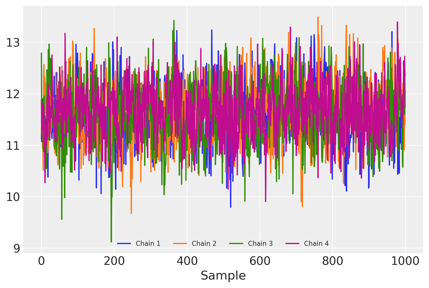
\(W\)(以及 \(F\)!)现在在采样器链之间的后验分布条目相同,尽管显然仍存在一些自相关。
因为F中的\(k \times n\)个参数都需要被采样,对于非常大的n,采样可能会变得非常昂贵。此外,观测数据点\(X_i\)与相关联的潜在值\(F_i\)之间的联系意味着无法进行带有小批量处理的流式推理。
这个可扩展性问题可以通过从模型中积分出 \(F\) 来进行分析解决。通过这样做,我们将任何关于 \(F_i\) 的个别值的计算推迟到以后。因此,这种方法通常被称为 摊销推理。然而,这固定了 \(F\) 的先验,从而减少了建模的灵活性。按照 \(F_{ij} \sim \mathcal{N}(0, I)\) 的规定,我们有:
\(X|WF \sim \mathcal{N}(WF, \sigma^2 I).\)
因此,我们可以将 \(X\) 写为
\(X = WF + \sigma I \epsilon,\)
其中 \(\epsilon \sim \mathcal{N}(0, I)\)。 固定 \(W\) 但将 \(F\) 和 \(\epsilon\) 视为随机变量,两者 \(\sim\mathcal{N}(0, I)\),我们看到 \(X\) 是两个多元正态变量的和,均值为 \(0\),协方差分别为 \(WW^T\) 和 \(\sigma^2 I\)。因此
\(X|W \sim \mathcal{N}(0, WW^T + \sigma^2 I )\).
with pm.Model(coords=coords) as PPCA_amortized:
    W = makeW(d, k, ("observed_columns", "latent_columns"))
    sigma = pm.HalfNormal("sigma", 1.0)
    cov = W @ W.T + sigma**2 * pt.eye(d)
    # MvNormal parametrizes covariance of columns, so transpose Y
    X = pm.MvNormal("X", 0.0, cov=cov, observed=Y.T, dims=("rows", "observed_columns"))
    trace_amortized = pm.sample(tune=30, draws=100, random_seed=rng)
Only 100 samples in chain.
Auto-assigning NUTS sampler...
Initializing NUTS using jitter+adapt_diag...
Multiprocess sampling (4 chains in 4 jobs)
NUTS: [W_z, W_b, sigma]
Sampling 4 chains for 30 tune and 100 draw iterations (120 + 400 draws total) took 52 seconds.
The rhat statistic is larger than 1.01 for some parameters. This indicates problems during sampling. See https://arxiv.org/abs/1903.08008 for details
The effective sample size per chain is smaller than 100 for some parameters.  A higher number is needed for reliable rhat and ess computation. See https://arxiv.org/abs/1903.08008 for details
不幸的是,该模型的采样非常慢,大概是因为计算MvNormal的对数概率需要对协方差矩阵进行求逆。然而,\(F\)的显式积分也使得可以对观测值进行批处理,以加快ADVI和FullRankADVI近似的计算速度。
coords["observed_columns2"] = coords["observed_columns"]
with pm.Model(coords=coords) as PPCA_amortized_batched:
    W = makeW(d, k, ("observed_columns", "latent_columns"))
    Y_mb = pm.Minibatch(
        Y.T, batch_size=50
    )  # MvNormal parametrizes covariance of columns, so transpose Y
    sigma = pm.HalfNormal("sigma", 1.0)
    cov = W @ W.T + sigma**2 * pt.eye(d)
    X = pm.MvNormal("X", 0.0, cov=cov, observed=Y_mb)
    trace_vi = pm.fit(n=50000, method="fullrank_advi", obj_n_mc=1).sample()
Finished [100%]: Average Loss = 1,759.7
/home/erik/miniforge3/envs/pymc_env/lib/python3.11/site-packages/pymc/backends/arviz.py:65: UserWarning: Could not extract data from symbolic observation X
  warnings.warn(f"Could not extract data from symbolic observation {obs}")
结果#
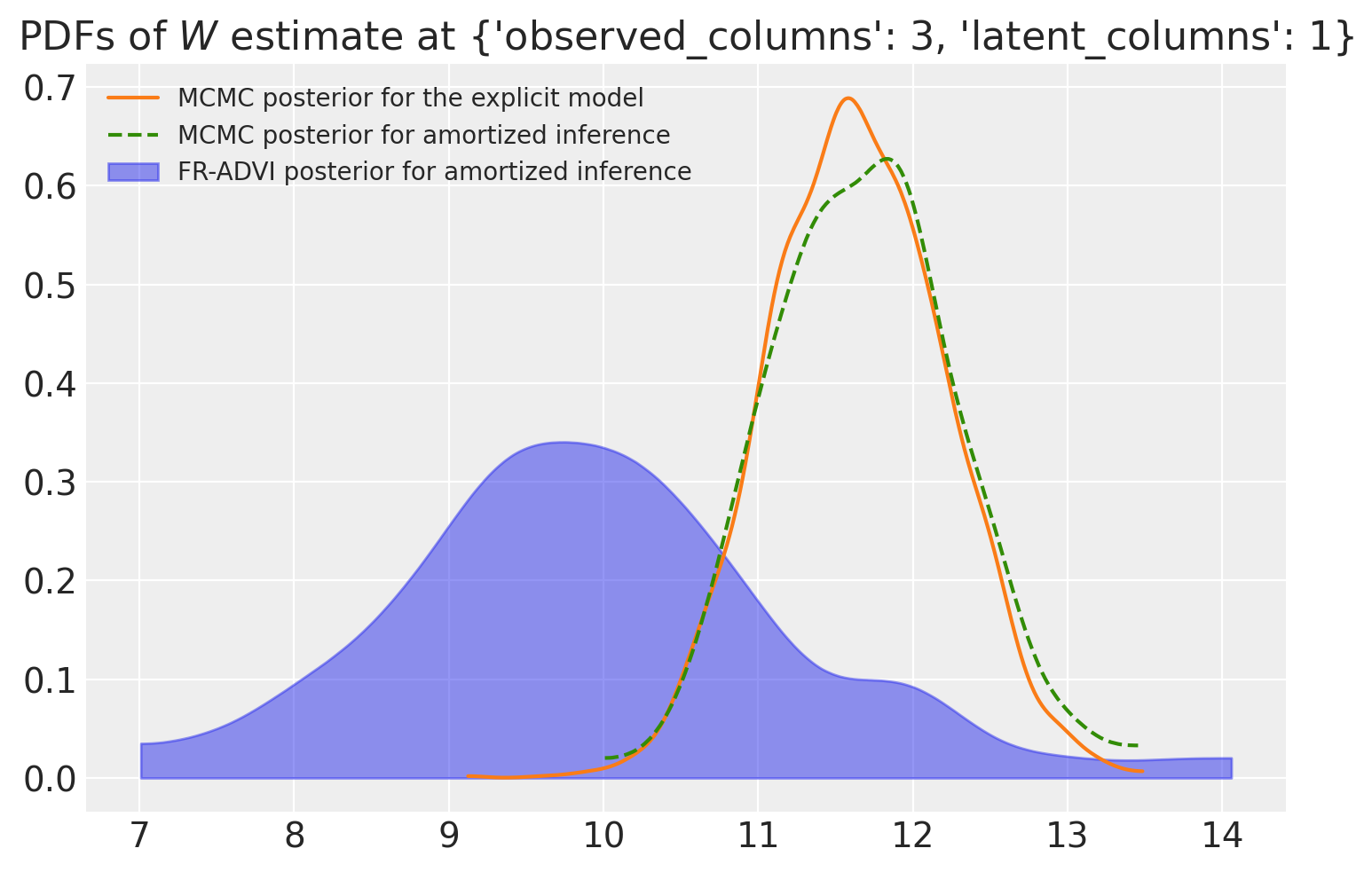
当我们比较使用MCMC和VI计算的后验概率时,我们发现(至少对于我们正在观察的这个特定参数)这两个分布是接近的,但它们的均值有所不同。两个MCMC后验概率彼此之间非常一致,而ADVI估计也相差不远。
col_selection = dict(observed_columns=3, latent_columns=1)

ax = az.plot_kde(
    trace.posterior["W"].sel(**col_selection).values,
    label="MCMC posterior for the explicit model".format(0),
    plot_kwargs={"color": f"C{1}"},
)

az.plot_kde(
    trace_amortized.posterior["W"].sel(**col_selection).values,
    label="MCMC posterior for amortized inference",
    plot_kwargs={"color": f"C{2}", "linestyle": "--"},
)


az.plot_kde(
    trace_vi.posterior["W"].sel(**col_selection).squeeze().values,
    label="FR-ADVI posterior for amortized inference",
    plot_kwargs={"alpha": 0},
    fill_kwargs={"alpha": 0.5, "color": f"C{0}"},
)


ax.set_title(rf"PDFs of $W$ estimate at {col_selection}")
ax.legend(loc="upper left", fontsize=10);
事后识别 F#
矩阵 \(F\) 通常是因子分析中感兴趣的对象,并且经常用作降维的特征矩阵。然而,\(F\) 已经被边缘化,以便更容易拟合模型;现在我们需要它回来。转换
\(X|WF \sim \mathcal{N}(WF, \sigma^2)\)
进入
\((W^TW)^{-1}W^T X|W,F \sim \mathcal{N}(F, \sigma^2(W^TW)^{-1})\)
我们将\(F\)表示为具有已知协方差矩阵的多变量正态分布的均值。使用先验\( F \sim \mathcal{N}(0, I) \)并根据共轭先验的表达式进行更新,我们得到
\( F | X, W \sim \mathcal{N}(\mu_F, \Sigma_F) \),
哪里
\(\mu_F = \left(I + \sigma^{-2} W^T W\right)^{-1} \sigma^{-2} W^T X\)
\(\Sigma_F = \left(I + \sigma^{-2} W^T W\right)^{-1}\)
对于在轨迹中找到的每个\(W\)和\(X\)的值,我们现在从这个分布中抽取一个样本。
# configure xarray-einstats
def get_default_dims(dims, dims2):
    proposed_dims = [dim for dim in dims if dim not in {"chain", "draw"}]
    assert len(proposed_dims) == 2
    if dims2 is None:
        return proposed_dims


linalg.get_default_dims = get_default_dims
post = trace_vi.posterior
obs = trace.observed_data

WW = linalg.matmul(
    post["W"], post["W"], dims=("latent_columns", "observed_columns", "latent_columns")
)

# Constructing an identity matrix following https://einstats.python.arviz.org/en/latest/tutorials/np_linalg_tutorial_port.html
I = xr.zeros_like(WW)
idx = xr.DataArray(WW.coords["latent_columns"])
I.loc[{"latent_columns": idx, "latent_columns2": idx}] = 1
Sigma_F = linalg.inv(I + post["sigma"] ** (-2) * WW)
X_transform = linalg.matmul(
    Sigma_F,
    post["sigma"] ** (-2) * post["W"],
    dims=("latent_columns2", "latent_columns", "observed_columns"),
)
mu_F = xr.dot(X_transform, obs["X"], dims="observed_columns").rename(
    latent_columns2="latent_columns"
)
Sigma_chol = linalg.cholesky(Sigma_F)
norm_dist = XrContinuousRV(sp.stats.norm, xr.zeros_like(mu_F))  # the zeros_like defines the shape
F_sampled = mu_F + linalg.matmul(
    post["sigma"] * Sigma_F,
    norm_dist.rvs(),
    dims=(("latent_columns", "latent_columns2"), ("latent_columns", "rows")),
)
与原始数据的比较#
为了检查我们的模型对原始数据的捕捉程度,我们将测试从采样的 \(W\) 和 \(F\) 矩阵中重建数据的准确性。对于 \(Y\) 的每个元素,我们绘制了基于模型重建的值 \(X = W F\) 的均值和标准差。
X_sampled_amortized = linalg.matmul(
    post["W"],
    F_sampled,
    dims=("observed_columns", "latent_columns", "rows"),
)
reconstruction_mean = X_sampled_amortized.mean(dim=("chain", "draw")).values
reconstruction_sd = X_sampled_amortized.std(dim=("chain", "draw")).values
plt.errorbar(
    Y.ravel(),
    reconstruction_mean.ravel(),
    yerr=reconstruction_sd.ravel(),
    marker=".",
    ls="none",
    alpha=0.3,
)

slope, intercept, r_value, p_value, std_err = sp.stats.linregress(
    Y.ravel(), reconstruction_mean.ravel()
)
plt.plot(
    [Y.min(), Y.max()],
    np.array([Y.min(), Y.max()]) * slope + intercept,
    "k--",
    label=f"Linear regression for the mean, R²={r_value**2:.2f}",
)
plt.plot([Y.min(), Y.max()], [Y.min(), Y.max()], "k:", label="Perfect reconstruction")

plt.xlabel("Elements of Y")
plt.ylabel("Model reconstruction")
plt.legend(loc="upper left");
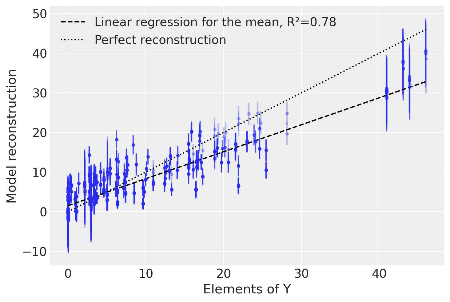
我们发现,尽管只使用了两个潜在因子而不是实际的四个,我们的模型在捕捉原始数据的变异方面做得相当不错。
水印#
%load_ext watermark
%watermark -n -u -v -iv -w
Last updated: Wed Dec 27 2023

Python implementation: CPython
Python version       : 3.11.7
IPython version      : 8.16.0

pytensor       : 2.18.3
scipy          : 1.11.4
arviz          : 0.16.1
seaborn        : 0.12.2
numpy          : 1.26.2
pymc           : 5.10.2
xarray         : 2023.12.0
xarray_einstats: 0.6.0
matplotlib     : 3.8.2

Watermark: 2.4.3
许可证声明#
本示例库中的所有笔记本均在MIT许可证下提供,该许可证允许修改和重新分发,前提是保留版权和许可证声明。
引用 PyMC 示例#
要引用此笔记本,请使用Zenodo为pymc-examples仓库提供的DOI。
重要
许多笔记本是从其他来源改编的:博客、书籍……在这种情况下,您应该引用原始来源。
同时记得引用代码中使用的相关库。
这是一个BibTeX的引用模板:
@incollection{citekey,
  author    = "<notebook authors, see above>",
  title     = "<notebook title>",
  editor    = "PyMC Team",
  booktitle = "PyMC examples",
  doi       = "10.5281/zenodo.5654871"
}
渲染后可能看起来像: