采样器统计信息

import arviz as az
import matplotlib.pyplot as plt
import numpy as np
import pandas as pd
import pymc as pm

%matplotlib inline

print(f"Running on PyMC v{pm.__version__}")

WARNING (pytensor.tensor.blas): Using NumPy C-API based implementation for BLAS functions.

Running on PyMC v4.0.0b6

az.style.use("arviz-darkgrid")
plt.rcParams["figure.constrained_layout.use"] = False

当检查收敛性或调试行为异常的采样器时，通常有助于更仔细地查看采样器正在执行的操作。为此，一些采样器会为每个生成的样本导出统计信息。

作为一个简单的例子，我们从标准正态分布中进行采样：

model = pm.Model()
with model:
    mu1 = pm.Normal("mu1", mu=0, sigma=1, shape=10)

with model:
    step = pm.NUTS()
    idata = pm.sample(2000, tune=1000, init=None, step=step, chains=4)

Multiprocess sampling (4 chains in 2 jobs)
NUTS: [mu1]

100.00% [12000/12000 00:06<00:00 Sampling 4 chains, 0 divergences]

Sampling 4 chains for 1_000 tune and 2_000 draw iterations (4_000 + 8_000 draws total) took 7 seconds.

• 注意: NUTS 提供了以下统计信息（这些是采样器使用的内部统计信息，在使用 PyMC 时您不需要对它们做任何操作，要了解更多信息，请参阅 pymc.NUTS。

idata.sample_stats

<xarray.Dataset>
Dimensions:             (chain: 4, draw: 2000)
Coordinates:
  * chain               (chain) int64 0 1 2 3
  * draw                (draw) int64 0 1 2 3 4 5 ... 1995 1996 1997 1998 1999
Data variables: (12/13)
    lp                  (chain, draw) float64 -17.41 -11.12 ... -13.76 -12.35
    perf_counter_diff   (chain, draw) float64 0.0009173 0.0009097 ... 0.0006041
    acceptance_rate     (chain, draw) float64 0.8478 1.0 ... 0.8888 0.8954
    energy_error        (chain, draw) float64 0.3484 -1.357 ... -0.2306 -0.2559
    energy              (chain, draw) float64 21.75 18.45 16.03 ... 19.25 16.51
    tree_depth          (chain, draw) int64 2 2 2 2 2 2 2 2 ... 2 2 3 2 2 2 2 2
    ...                  ...
    diverging           (chain, draw) bool False False False ... False False
    step_size           (chain, draw) float64 0.8831 0.8831 ... 0.848 0.848
    n_steps             (chain, draw) float64 3.0 3.0 3.0 3.0 ... 3.0 3.0 3.0
    perf_counter_start  (chain, draw) float64 2.591e+05 2.591e+05 ... 2.591e+05
    process_time_diff   (chain, draw) float64 0.0009183 0.0009112 ... 0.0006032
    max_energy_error    (chain, draw) float64 0.3896 -1.357 ... 0.2427 0.303
Attributes:
    created_at:                 2022-05-31T19:50:21.571347
    arviz_version:              0.12.1
    inference_library:          pymc
    inference_library_version:  4.0.0b6
    sampling_time:              6.993547439575195
    tuning_steps:               1000

xarray.Dataset

• Dimensions:
  • chain: 4
  • draw: 2000
• Coordinates: (2)
  • chain
    (chain)
    int64
    0 1 2 3

    array([0, 1, 2, 3])

  • draw
    (draw)
    int64
    0 1 2 3 4 ... 1996 1997 1998 1999

    array([   0,    1,    2, ..., 1997, 1998, 1999])

• Data variables: (13)
  • lp
    (chain, draw)
    float64
    -17.41 -11.12 ... -13.76 -12.35

    array([[-17.41481817, -11.11746073, -14.00889121, ..., -14.62579449,
            -15.12640488, -14.92067376],
           [-11.79754517, -11.37321931, -12.41967116, ..., -15.0553557 ,
            -15.03960873, -11.84774166],
           [-14.40032205, -20.68972653, -13.74758915, ..., -15.20451325,
            -13.46400824, -14.82413174],
           [-13.44881972, -15.9252134 , -11.73013359, ..., -14.77629777,
            -13.75935262, -12.34852981]])

  • perf_counter_diff
    (chain, draw)
    float64
    0.0009173 0.0009097 ... 0.0006041

    array([[0.00091726, 0.00090966, 0.00090066, ..., 0.00086925, 0.00092221,
            0.00046417],
           [0.00092182, 0.00084332, 0.00081795, ..., 0.00048199, 0.00048006,
            0.00048616],
           [0.00050058, 0.00061117, 0.0005809 , ..., 0.00170264, 0.00124334,
            0.00069834],
           [0.00050844, 0.00052396, 0.00054123, ..., 0.00051385, 0.0005149 ,
            0.00060409]])

  • acceptance_rate
    (chain, draw)
    float64
    0.8478 1.0 0.5188 ... 0.8888 0.8954

    array([[0.84781696, 1.        , 0.5188267 , ..., 0.91934539, 0.85438787,
            0.76057673],
           [1.        , 0.81181648, 0.93142852, ..., 0.94123492, 0.75399724,
            0.93529202],
           [1.        , 0.29414685, 1.        , ..., 0.46697774, 0.83249289,
            0.65167911],
           [0.79107091, 0.56355851, 1.        , ..., 0.92367151, 0.8888214 ,
            0.89536079]])

  • energy_error
    (chain, draw)
    float64
    0.3484 -1.357 ... -0.2306 -0.2559

    array([[ 0.34837379, -1.3573709 ,  0.72431555, ...,  0.2857954 ,
             0.1180722 ,  0.03878686],
           [-0.15890021, -0.10739294,  0.2229767 , ...,  0.01717362,
            -0.13001742, -0.69487895],
           [-0.21978325,  1.47962416, -1.65668177, ...,  0.50839378,
            -0.41858308,  0.3440592 ],
           [-0.14333517,  0.51606888, -0.88905807, ...,  0.0211668 ,
            -0.23064281, -0.25594826]])

  • energy
    (chain, draw)
    float64
    21.75 18.45 16.03 ... 19.25 16.51

    array([[21.75076832, 18.45266859, 16.03241029, ..., 17.16983192,
            20.13659553, 23.01097321],
           [14.09025318, 15.15479489, 13.75490571, ..., 18.64000448,
            21.55766921, 19.64569656],
           [17.32485111, 25.19494315, 24.5830488 , ..., 21.14581229,
            20.19801996, 19.52502693],
           [22.87267199, 20.94006237, 16.61780155, ..., 19.3110406 ,
            19.24706179, 16.51436075]])

  • tree_depth
    (chain, draw)
    int64
    2 2 2 2 2 2 2 2 ... 2 2 3 2 2 2 2 2

    array([[2, 2, 2, ..., 3, 3, 2],
           [2, 2, 2, ..., 2, 2, 2],
           [2, 2, 2, ..., 3, 2, 2],
           [2, 2, 2, ..., 2, 2, 2]])

  • step_size_bar
    (chain, draw)
    float64
    0.9358 0.9358 ... 0.9276 0.9276

    array([[0.93583778, 0.93583778, 0.93583778, ..., 0.93583778, 0.93583778,
            0.93583778],
           [0.96472688, 0.96472688, 0.96472688, ..., 0.96472688, 0.96472688,
            0.96472688],
           [0.97413339, 0.97413339, 0.97413339, ..., 0.97413339, 0.97413339,
            0.97413339],
           [0.92757304, 0.92757304, 0.92757304, ..., 0.92757304, 0.92757304,
            0.92757304]])

  • diverging
    (chain, draw)
    bool
    False False False ... False False

    array([[False, False, False, ..., False, False, False],
           [False, False, False, ..., False, False, False],
           [False, False, False, ..., False, False, False],
           [False, False, False, ..., False, False, False]])

  • step_size
    (chain, draw)
    float64
    0.8831 0.8831 ... 0.848 0.848

    array([[0.88314133, 0.88314133, 0.88314133, ..., 0.88314133, 0.88314133,
            0.88314133],
           [0.98491061, 0.98491061, 0.98491061, ..., 0.98491061, 0.98491061,
            0.98491061],
           [0.79717973, 0.79717973, 0.79717973, ..., 0.79717973, 0.79717973,
            0.79717973],
           [0.84803742, 0.84803742, 0.84803742, ..., 0.84803742, 0.84803742,
            0.84803742]])

  • n_steps
    (chain, draw)
    float64
    3.0 3.0 3.0 3.0 ... 3.0 3.0 3.0 3.0

    array([[3., 3., 3., ..., 7., 7., 3.],
           [3., 3., 3., ..., 3., 3., 3.],
           [3., 3., 3., ..., 7., 3., 3.],
           [3., 3., 3., ..., 3., 3., 3.]])

  • perf_counter_start
    (chain, draw)
    float64
    2.591e+05 2.591e+05 ... 2.591e+05

    array([[259080.94794072, 259080.9491462 , 259080.95033726, ...,
            259082.86608642, 259082.86711713, 259082.86821631],
           [259080.90127503, 259080.90247671, 259080.90355453, ...,
            259082.70122436, 259082.70185994, 259082.70249527],
           [259083.94110883, 259083.94177995, 259083.94255876, ...,
            259085.68260603, 259085.68468606, 259085.68622814],
           [259084.07774306, 259084.07843519, 259084.07920939, ...,
            259085.84236159, 259085.8430168 , 259085.84369495]])

  • process_time_diff
    (chain, draw)
    float64
    0.0009183 0.0009112 ... 0.0006032

    array([[0.00091832, 0.00091119, 0.00090133, ..., 0.00086943, 0.00092247,
            0.00046421],
           [0.00092232, 0.00084386, 0.00081837, ..., 0.00048233, 0.0004802 ,
            0.00048617],
           [0.00050046, 0.00052388, 0.0005813 , ..., 0.00170327, 0.001244  ,
            0.00069857],
           [0.00050863, 0.00052436, 0.00054133, ..., 0.0005133 , 0.00051457,
            0.00060323]])

  • max_energy_error
    (chain, draw)
    float64
    0.3896 -1.357 ... 0.2427 0.303

    array([[ 0.3896375 , -1.3573709 ,  0.72431555, ...,  0.34345   ,
             0.42071847,  1.28485975],
           [-0.21887002,  0.50399625,  0.2229767 , ..., -0.78518544,
             1.03001369, -0.69487895],
           [-1.00930297,  1.47962416, -1.65668177, ...,  1.11431688,
             0.47088174,  0.88911589],
           [ 1.87193377,  1.14125086, -0.88905807, ...,  0.31397184,
             0.24269705,  0.30297649]])

• Attributes: (6)

  created_at :

  2022-05-31T19:50:21.571347

  arviz_version :

  0.12.1

  inference_library :

  pymc

  inference_library_version :

  4.0.0b6

  sampling_time :

  6.993547439575195

  tuning_steps :

  1000

样本统计变量定义如下：

• process_time_diff: 绘制样本所花费的时间，由python标准库time.process_time定义。这包括所有CPU时间，包括BLAS和OpenMP中的工作进程。

• step_size: 当前积分步长。

• diverging: (布尔值) 表示存在从起点和后续终止轨迹中能量偏差较大的蛙跳过渡。“较大”定义为 max_energy_error 超过阈值。

• lp: 模型的联合对数后验密度（直到一个加性常数）。

• energy: 接受提议的哈密顿能量的值（直到一个加性常数）。

• energy_error: 初始点和接受提议之间的哈密顿能量差异。

• perf_counter_diff: 绘制样本所需的时间，由Python标准库time.perf_counter定义（挂钟时间）。

• perf_counter_start: 在绘制计算开始时的时间.perf_counter值。

• n_steps: 计算的蛙跳步数。它与tree_depth相关，满足n_steps <= 2^tree_dept。

• max_energy_error: 在提议的树中，初始点与所有可能样本之间的哈密顿能量最大绝对差值。

• acceptance_rate: 提议树中所有可能样本的平均接受概率。

• step_size_bar: 当前已知的最佳步长。在调整样本之后，步长被设置为这个值。这个值应在调整过程中收敛。

• tree_depth: 平衡二叉树中树翻倍的次数。

需要注意的几点：

• 在转换为InferenceData时，NUTS使用的一些样本统计信息会被重命名，以遵循ArviZ 的命名约定，而有些则是特定于 PyMC3 的，并在生成的 InferenceData 对象中保留其内部的 PyMC3 名称。

• InferenceData 还存储了额外的信息，如日期、使用的版本、采样时间和调优步骤作为属性。

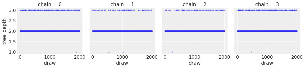
idata.sample_stats["tree_depth"].plot(col="chain", ls="none", marker=".", alpha=0.3);

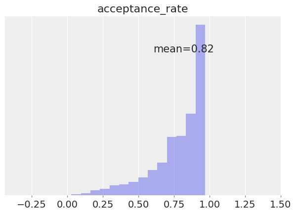
az.plot_posterior(
    idata, group="sample_stats", var_names="acceptance_rate", hdi_prob="hide", kind="hist"
);

我们检查是否存在任何分歧，如果存在，有多少？

idata.sample_stats["diverging"].sum()

<xarray.DataArray 'diverging' ()>
array(0)

xarray.DataArray

'diverging'

• 0

  array(0)

• Coordinates: (0)
• Attributes: (0)

在这种情况下，没有发现分歧。如果有任何分歧，请查看此笔记本以获取处理分歧的信息。

比较能量水平总体分布与相邻样本间能量变化通常很有用。理想情况下，它们应该非常相似：

az.plot_energy(idata, figsize=(6, 4));

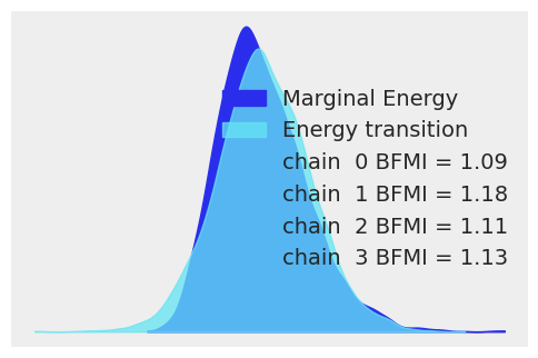
如果能量水平的整体分布具有更长的尾部，采样器的效率将迅速下降。

多个采样器

如果为同一模型使用了多个采样器（例如，用于连续变量和离散变量），导出的值将沿新轴合并或堆叠。

coords = {"step": ["BinaryMetropolis", "Metropolis"], "obs": ["mu1"]}
dims = {"accept": ["step"]}

with pm.Model(coords=coords) as model:
    mu1 = pm.Bernoulli("mu1", p=0.8)
    mu2 = pm.Normal("mu2", mu=0, sigma=1, dims="obs")

with model:
    step1 = pm.BinaryMetropolis([mu1])
    step2 = pm.Metropolis([mu2])
    idata = pm.sample(
        10000,
        init=None,
        step=[step1, step2],
        chains=4,
        tune=1000,
        idata_kwargs={"dims": dims, "coords": coords},
    )

Multiprocess sampling (4 chains in 2 jobs)
CompoundStep
>BinaryMetropolis: [mu1]
>Metropolis: [mu2]

100.00% [44000/44000 00:14<00:00 Sampling 4 chains, 0 divergences]

Sampling 4 chains for 1_000 tune and 10_000 draw iterations (4_000 + 40_000 draws total) took 15 seconds.

list(idata.sample_stats.data_vars)

['p_jump', 'scaling', 'accepted', 'accept']

两个采样器都导出 accept，因此我们为每个采样器获得一个接受概率：

az.plot_posterior(
    idata,
    group="sample_stats",
    var_names="accept",
    hdi_prob="hide",
    kind="hist",
);

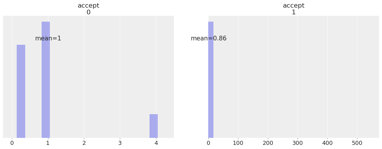
我们注意到accept有时会取到非常高的值（从低概率区域跳到高概率区域）。

# Range of accept values
idata.sample_stats["accept"].max("draw") - idata.sample_stats["accept"].min("draw")

<xarray.DataArray 'accept' (chain: 4, accept_dim_0: 2)>
array([[  3.75      , 573.3089824 ],
       [  3.75      , 184.17692429],
       [  3.75      , 194.61242919],
       [  3.75      ,  88.51883672]])
Coordinates:
  * chain         (chain) int64 0 1 2 3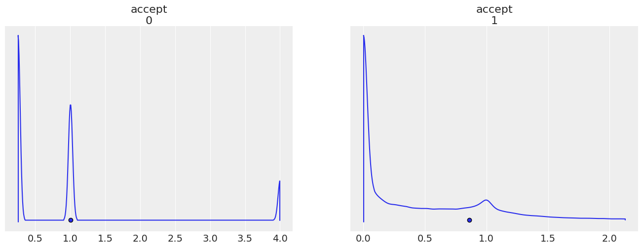
  * accept_dim_0  (accept_dim_0) int64 0 1

xarray.DataArray

'accept'

• chain: 4
• accept_dim_0: 2

• 3.75 573.3 3.75 184.2 3.75 194.6 3.75 88.52

  array([[  3.75      , 573.3089824 ],
         [  3.75      , 184.17692429],
         [  3.75      , 194.61242919],
         [  3.75      ,  88.51883672]])

• Coordinates: (2)
  • chain
    (chain)
    int64
    0 1 2 3

    array([0, 1, 2, 3])

  • accept_dim_0
    (accept_dim_0)
    int64
    0 1

    array([0, 1])

• Attributes: (0)

# We can try plotting the density and view the high density intervals to understand the variable better
az.plot_density(
    idata,
    group="sample_stats",
    var_names="accept",
    point_estimate="mean",
);

作者

• 由Meenal Jhajharia于2021年4月更新（pymc-examples#95）

• 由Christian Luhmann于2022年5月更新至v4（pymc-examples#338）

水印

%load_ext watermark
%watermark -n -u -v -iv -w

Last updated: Tue May 31 2022

Python implementation: CPython
Python version       : 3.10.4
IPython version      : 8.4.0

arviz     : 0.12.1
numpy     : 1.23.0rc2
pymc      : 4.0.0b6
matplotlib: 3.5.2
pandas    : 1.4.2

Watermark: 2.3.1

许可证声明

本示例库中的所有笔记本均在MIT许可证下提供，该许可证允许修改和重新分发，前提是保留版权和许可证声明。

引用 PyMC 示例

要引用此笔记本，请使用Zenodo为pymc-examples仓库提供的DOI。

重要

许多笔记本是从其他来源改编的：博客、书籍……在这种情况下，您应该引用原始来源。

同时记得引用代码中使用的相关库。

这是一个BibTeX的引用模板：

@incollection{citekey,
  author    = "<notebook authors, see above>",
  title     = "<notebook title>",
  editor    = "PyMC Team",
  booktitle = "PyMC examples",
  doi       = "10.5281/zenodo.5654871"
}

渲染后可能看起来像：