异方差高斯过程#
我们通常可以将模型中的不确定性来源分为两类。“Aleatoric”不确定性(源自拉丁语中的骰子或随机性)源于我们系统固有的变异性。“Epistemic”不确定性(源自希腊语中的知识)源于我们的观察在整个感兴趣领域中的分布方式。
高斯过程(GP)模型是一种强大的工具,可以捕捉这两种不确定性来源。通过考虑满足协方差核和数据指定条件的所有函数的分布,这些模型在观测点附近表现出较低的认知不确定性,而在远离观测点的地方表现出较高的认知不确定性。为了结合偶然不确定性,标准GP模型假设在整个域内添加具有恒定幅度的白噪声。然而,这种“同方差”模型如果在某些区域具有比其他区域更高的方差,则可能无法很好地表示您的系统。在其他领域中,这在实验科学中尤为常见,其中变化的实验参数可以影响响应的大小和变异性。明确地结合噪声对输入和输出的依赖性(以及相互依赖性)可以更好地理解平均行为,并为优化提供更具信息量的景观,例如。
本笔记本将通过几种方法来处理具有GP的异方差建模。我们将使用代表在系统上的一系列输入值处(独立)重复测量的玩具数据,其中噪声的大小随响应变量增加。我们将从简单的建模方法开始,例如在每个点上拟合一个GP到均值,并根据每个点的方差进行加权(如果在已知不确定性的方法中进行单个测量,这可能是有用的),将其与典型的同方差GP进行对比。然后,我们将构建一个模型,使用一个潜在的GP来建模响应均值,并使用第二个(独立的)潜在GP来建模响应方差。为了提高该模型的效率和可扩展性,我们将在稀疏框架中重新构建它。最后,我们将使用协区域核来允许噪声和平均响应之间的相关性。
数据#
import arviz as az
import matplotlib.pyplot as plt
import numpy as np
import pymc3 as pm
import theano.tensor as tt

from scipy.spatial.distance import pdist

%config InlineBackend.figure_format ='retina'
%load_ext watermark
SEED = 2020
rng = np.random.default_rng(SEED)
az.style.use("arviz-darkgrid")
def signal(x):
return x / 2 + np.sin(2 * np.pi * x) / 5
def noise(y):
return np.exp(y) / 20
X = np.linspace(0.1, 1, 20)[:, None]
X = np.vstack([X, X + 2])
X_ = X.flatten()
y = signal(X_)
σ_fun = noise(y)
y_err = rng.lognormal(np.log(σ_fun), 0.1)
y_obs = rng.normal(y, y_err, size=(5, len(y)))
y_obs_ = y_obs.T.flatten()
X_obs = np.tile(X.T, (5, 1)).T.reshape(-1, 1)
X_obs_ = X_obs.flatten()
idx = np.tile(np.array([i for i, _ in enumerate(X_)]), (5, 1)).T.flatten()
Xnew = np.linspace(-0.15, 3.25, 100)[:, None]
Xnew_ = Xnew.flatten()
ynew = signal(Xnew)
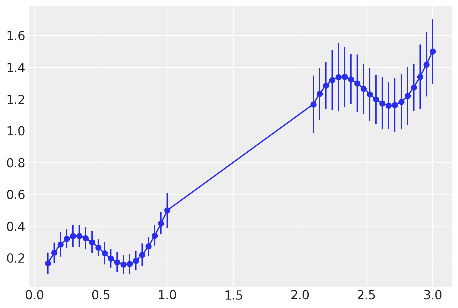
plt.plot(X, y, "C0o")
plt.errorbar(X_, y, y_err, color="C0")
<ErrorbarContainer object of 3 artists>
辅助函数和绘图函数#
def get_ℓ_prior(points):
    """Calculates mean and sd for InverseGamma prior on lengthscale"""
    distances = pdist(points[:, None])
    distinct = distances != 0
    ℓ_l = distances[distinct].min() if sum(distinct) > 0 else 0.1
    ℓ_u = distances[distinct].max() if sum(distinct) > 0 else 1
    ℓ_σ = max(0.1, (ℓ_u - ℓ_l) / 6)
    ℓ_μ = ℓ_l + 3 * ℓ_σ
    return ℓ_μ, ℓ_σ


ℓ_μ, ℓ_σ = [stat for stat in get_ℓ_prior(X_)]
def plot_inducing_points(ax):
    yl = ax.get_ylim()
    yu = -np.subtract(*yl) * 0.025 + yl[0]
    ax.plot(Xu, np.full(Xu.shape, yu), "xk", label="Inducing Points")
    ax.legend(loc="upper left")


def get_quantiles(samples, quantiles=[2.5, 50, 97.5]):
    return [np.percentile(samples, p, axis=0) for p in quantiles]


def plot_mean(ax, mean_samples):
    """Plots the median and 95% CI from samples of the mean

    Note that, although each individual GP exhibits a normal distribution at each point
    (by definition), we are sampling from a mixture of GPs defined by the posteriors of
    our hyperparameters. As such, we use percentiles rather than mean +/- stdev to
    represent the spread of predictions from our models.
    """
    l, m, u = get_quantiles(mean_samples)
    ax.plot(Xnew, m, "C0", label="Median")
    ax.fill_between(Xnew_, l, u, facecolor="C0", alpha=0.5, label="95% CI")

    ax.plot(Xnew, ynew, "--k", label="Mean Function")
    ax.plot(X, y, "C1.", label="Observed Means")
    ax.set_title("Mean Behavior")
    ax.legend(loc="upper left")


def plot_var(ax, var_samples):
    """Plots the median and 95% CI from samples of the variance"""
    if var_samples.squeeze().ndim == 1:
        ax.plot(Xnew, var_samples, "C0", label="Median")
    else:
        l, m, u = get_quantiles(var_samples)
        ax.plot(Xnew, m, "C0", label="Median")
        ax.fill_between(Xnew.flatten(), l, u, facecolor="C0", alpha=0.5, label="95% CI")
    ax.plot(Xnew, noise(signal(Xnew_)) ** 2, "--k", label="Noise Function")
    ax.plot(X, y_err**2, "C1.", label="Observed Variance")
    ax.set_title("Variance Behavior")
    ax.legend(loc="upper left")


def plot_total(ax, mean_samples, var_samples=None, bootstrap=True, n_boots=100):
    """Plots the overall mean and variance of the aggregate system

    We can represent the overall uncertainty via explicitly sampling the underlying normal
    distributrions (with `bootstrap=True`) or as the mean +/- the standard deviation from
    the Law of Total Variance. For systems with many observations, there will likely be
    little difference, but in cases with few observations and informative priors, plotting
    the percentiles will likely give a more accurate representation.
    """

    if (var_samples is None) or (var_samples.squeeze().ndim == 1):
        samples = mean_samples
        l, m, u = get_quantiles(samples)
        ax.plot(Xnew, m, "C0", label="Median")
    elif bootstrap:
        # Estimate the aggregate behavior using samples from each normal distribution in the posterior
        samples = (
            rng.normal(
                mean_samples.T[:, :, None],
                np.sqrt(var_samples).T[:, :, None],
                (*mean_samples.T.shape, n_boots),
            )
            .reshape(len(Xnew_), -1)
            .T
        )
        l, m, u = get_quantiles(samples)
        ax.plot(Xnew, m, "C0", label="Median")
    else:
        m = mean_samples.mean(axis=0)
        ax.plot(Xnew, m, "C0", label="Mean")
        sd = np.sqrt(mean_samples.var(axis=0) + var_samples.mean(axis=0))
        l, u = m - 2 * sd, m + 2 * sd

    ax.fill_between(Xnew.flatten(), l, u, facecolor="C0", alpha=0.5, label="Total 95% CI")

    ax.plot(Xnew, ynew, "--k", label="Mean Function")
    ax.plot(X_obs, y_obs_, "C1.", label="Observations")
    ax.set_title("Aggregate Behavior")
    ax.legend(loc="upper left")
同方差高斯过程#
首先,我们使用PyMC3的边际似然实现来拟合一个标准的同方差高斯过程。在本笔记本中,我们将使用Michael Betancourt建议的长度尺度信息先验。我们可以使用pm.find_MAP()和.predict来进行更快的推断和预测,结果相似,但为了与其他模型进行直接比较,我们将使用NUTS和.conditional,它们运行得足够快。
with pm.Model() as model_hm:
    ℓ = pm.InverseGamma("ℓ", mu=ℓ_μ, sigma=ℓ_σ)
    η = pm.Gamma("η", alpha=2, beta=1)
    cov = η**2 * pm.gp.cov.ExpQuad(input_dim=1, ls=ℓ)

    gp_hm = pm.gp.Marginal(cov_func=cov)

    σ = pm.Exponential("σ", lam=1)

    ml_hm = gp_hm.marginal_likelihood("ml_hm", X=X_obs, y=y_obs_, noise=σ)

    trace_hm = pm.sample(return_inferencedata=True, random_seed=SEED)

with model_hm:
    mu_pred_hm = gp_hm.conditional("mu_pred_hm", Xnew=Xnew)
    noisy_pred_hm = gp_hm.conditional("noisy_pred_hm", Xnew=Xnew, pred_noise=True)
    samples_hm = pm.sample_posterior_predictive(trace_hm, var_names=["mu_pred_hm", "noisy_pred_hm"])
Auto-assigning NUTS sampler...
Initializing NUTS using jitter+adapt_diag...
Multiprocess sampling (4 chains in 4 jobs)
NUTS: [σ, η, ℓ]
Sampling 4 chains for 1_000 tune and 1_000 draw iterations (4_000 + 4_000 draws total) took 112 seconds.
_, axs = plt.subplots(1, 3, figsize=(18, 4))
mu_samples = samples_hm["mu_pred_hm"]
noisy_samples = samples_hm["noisy_pred_hm"]
plot_mean(axs[0], mu_samples)
plot_var(axs[1], noisy_samples.var(axis=0))
plot_total(axs[2], noisy_samples)
在这里,我们在左侧绘制了我们对平均行为的理解以及相应的认知不确定性,在中间绘制了我们对方差或偶然不确定性的理解,并在右侧整合了所有不确定性来源。该模型很好地捕捉了平均行为,但正如预期的那样,我们可以看到它在较低范围内高估了噪声,而在较高范围内低估了噪声。
方差加权GP#
建模异方差系统的最简单方法是沿域的每个点拟合一个GP在均值上,并将标准差作为权重提供。
with pm.Model() as model_wt:
    ℓ = pm.InverseGamma("ℓ", mu=ℓ_μ, sigma=ℓ_σ)
    η = pm.Gamma("η", alpha=2, beta=1)
    cov = η**2 * pm.gp.cov.ExpQuad(input_dim=1, ls=ℓ)

    gp_wt = pm.gp.Marginal(cov_func=cov)

    ml_wt = gp_wt.marginal_likelihood("ml_wt", X=X, y=y, noise=y_err)

    trace_wt = pm.sample(return_inferencedata=True, random_seed=SEED)

with model_wt:
    mu_pred_wt = gp_wt.conditional("mu_pred_wt", Xnew=Xnew)
    samples_wt = pm.sample_posterior_predictive(trace_wt, var_names=["mu_pred_wt"])
Auto-assigning NUTS sampler...
Initializing NUTS using jitter+adapt_diag...
Multiprocess sampling (4 chains in 4 jobs)
NUTS: [η, ℓ]
Sampling 4 chains for 1_000 tune and 1_000 draw iterations (4_000 + 4_000 draws total) took 18 seconds.
_, axs = plt.subplots(1, 3, figsize=(18, 4))
mu_samples = samples_wt["mu_pred_wt"]
plot_mean(axs[0], mu_samples)
axs[0].errorbar(X_, y, y_err, ls="none", color="C1", label="STDEV")
plot_var(axs[1], mu_samples.var(axis=0))
plot_total(axs[2], mu_samples)
这种方法在整体不确定性中捕捉到了比同方差高斯过程(homoskedastic GP)稍多的细微差别,但仍然低估了两个观测机制内的方差。请注意,该模型显示的方差纯粹是认知性的:我们对平均行为的理解是根据观测中的不确定性加权的,但我们没有包含一个组件来解释偶然性噪声。
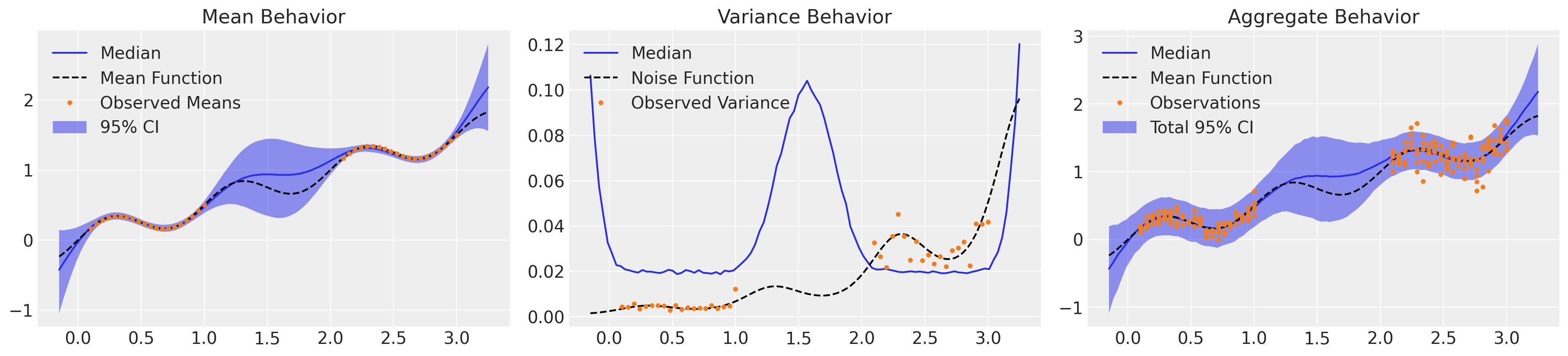
异方差GP:潜在方差模型#
现在让我们通过PyMC3的Latent实现将均值和对数方差分别建模为独立的GP,并将两者输入到Normal似然中。请注意,我们在各个协方差中添加了少量的对角噪声,以稳定它们以便进行逆运算。
with pm.Model() as model_ht:
    ℓ = pm.InverseGamma("ℓ", mu=ℓ_μ, sigma=ℓ_σ)
    η = pm.Gamma("η", alpha=2, beta=1)
    cov = η**2 * pm.gp.cov.ExpQuad(input_dim=1, ls=ℓ) + pm.gp.cov.WhiteNoise(sigma=1e-6)

    gp_ht = pm.gp.Latent(cov_func=cov)
    μ_f = gp_ht.prior("μ_f", X=X_obs)

    σ_ℓ = pm.InverseGamma("σ_ℓ", mu=ℓ_μ, sigma=ℓ_σ)
    σ_η = pm.Gamma("σ_η", alpha=2, beta=1)
    σ_cov = σ_η**2 * pm.gp.cov.ExpQuad(input_dim=1, ls=σ_ℓ) + pm.gp.cov.WhiteNoise(sigma=1e-6)

    σ_gp = pm.gp.Latent(cov_func=σ_cov)
    lg_σ_f = σ_gp.prior("lg_σ_f", X=X_obs)
    σ_f = pm.Deterministic("σ_f", pm.math.exp(lg_σ_f))

    lik_ht = pm.Normal("lik_ht", mu=μ_f, sd=σ_f, observed=y_obs_)

    trace_ht = pm.sample(target_accept=0.95, chains=2, return_inferencedata=True, random_seed=SEED)

with model_ht:
    μ_pred_ht = gp_ht.conditional("μ_pred_ht", Xnew=Xnew)
    lg_σ_pred_ht = σ_gp.conditional("lg_σ_pred_ht", Xnew=Xnew)
    samples_ht = pm.sample_posterior_predictive(trace_ht, var_names=["μ_pred_ht", "lg_σ_pred_ht"])
Auto-assigning NUTS sampler...
Initializing NUTS using jitter+adapt_diag...
Multiprocess sampling (2 chains in 4 jobs)
NUTS: [lg_σ_f_rotated_, σ_η, σ_ℓ, μ_f_rotated_, η, ℓ]
Sampling 2 chains for 1_000 tune and 1_000 draw iterations (2_000 + 2_000 draws total) took 7652 seconds.
There were 9 divergences after tuning. Increase `target_accept` or reparameterize.
There were 17 divergences after tuning. Increase `target_accept` or reparameterize.
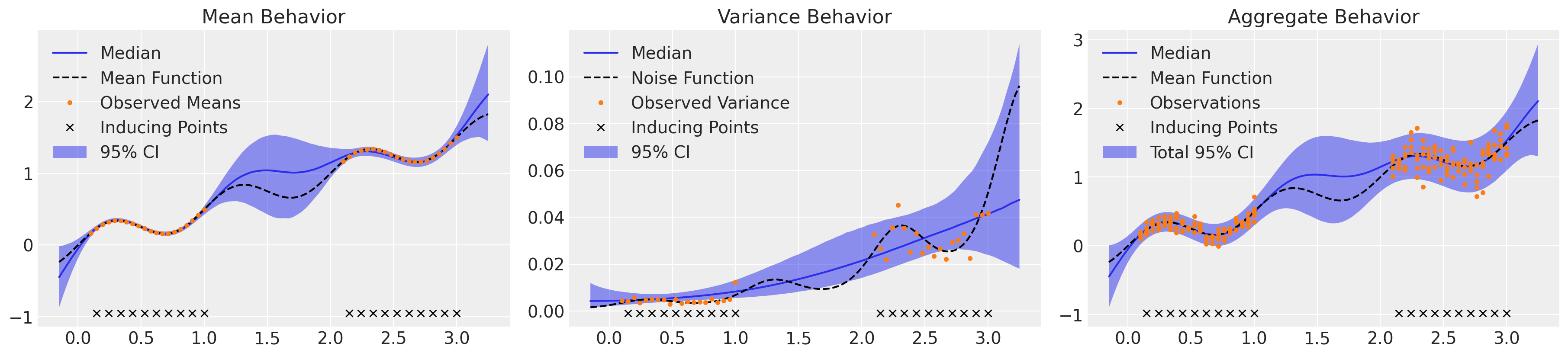
_, axs = plt.subplots(1, 3, figsize=(18, 4))
μ_samples = samples_ht["μ_pred_ht"]
σ_samples = np.exp(samples_ht["lg_σ_pred_ht"])
plot_mean(axs[0], μ_samples)
plot_var(axs[1], σ_samples**2)
plot_total(axs[2], μ_samples, σ_samples**2)
看起来好多了!我们已经准确地捕捉到了系统平均行为,并理解了方差中的潜在趋势,同时考虑了适当的不确定性。关键的是,模型的整体行为结合了认知不确定性和偶然不确定性,并且我们观察到的约5%的数据落在2σ带之外,这些数据在域内或多或少均匀分布。然而,这花费了超过两个小时的时间来采样仅4k的NUTS迭代。由于所需的矩阵求逆的代价,高斯过程在处理大数据集时以效率低下而闻名。让我们使用稀疏近似来重新构建这个模型。
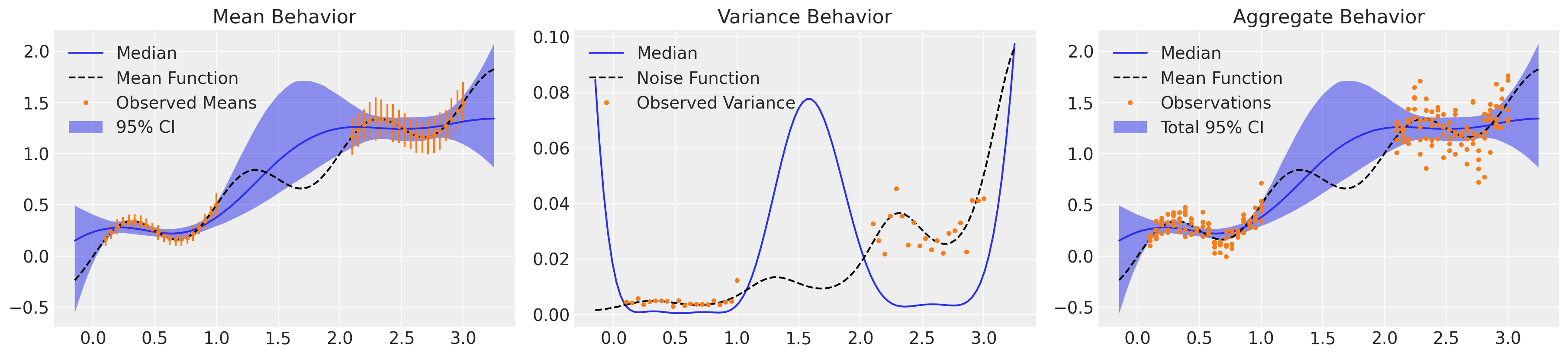
稀疏异方差GP#
稀疏近似于GPs使用一小部分诱导点来条件化模型,极大地提高了推理速度,并在一定程度上改善了内存消耗。PyMC3目前还没有实现稀疏潜在GPs(尚未),但我们可以快速地使用Bill Engel的DTC潜在GP示例来实现。这些诱导点可以通过多种方式指定,例如通过流行的k-means初始化或甚至作为模型的一部分进行优化,但由于我们的观察值均匀分布,我们可以简单地使用我们唯一输入值的一个子集。
class SparseLatent:
    def __init__(self, cov_func):
        self.cov = cov_func

    def prior(self, name, X, Xu):
        Kuu = self.cov(Xu)
        self.L = pm.gp.util.cholesky(pm.gp.util.stabilize(Kuu))

        self.v = pm.Normal(f"u_rotated_{name}", mu=0.0, sd=1.0, shape=len(Xu))
        self.u = pm.Deterministic(f"u_{name}", tt.dot(self.L, self.v))

        Kfu = self.cov(X, Xu)
        self.Kuiu = tt.slinalg.solve_upper_triangular(
            self.L.T, tt.slinalg.solve_lower_triangular(self.L, self.u)
        )
        self.mu = pm.Deterministic(f"mu_{name}", tt.dot(Kfu, self.Kuiu))
        return self.mu

    def conditional(self, name, Xnew, Xu):
        Ksu = self.cov(Xnew, Xu)
        mus = tt.dot(Ksu, self.Kuiu)
        tmp = tt.slinalg.solve_lower_triangular(self.L, Ksu.T)
        Qss = tt.dot(tmp.T, tmp)  # Qss = tt.dot(tt.dot(Ksu, tt.nlinalg.pinv(Kuu)), Ksu.T)
        Kss = self.cov(Xnew)
        Lss = pm.gp.util.cholesky(pm.gp.util.stabilize(Kss - Qss))
        mu_pred = pm.MvNormal(name, mu=mus, chol=Lss, shape=len(Xnew))
        return mu_pred
# Explicitly specify inducing points by downsampling our input vector
Xu = X[1::2]

with pm.Model() as model_hts:
    ℓ = pm.InverseGamma("ℓ", mu=ℓ_μ, sigma=ℓ_σ)
    η = pm.Gamma("η", alpha=2, beta=1)
    cov = η**2 * pm.gp.cov.ExpQuad(input_dim=1, ls=ℓ)

    μ_gp = SparseLatent(cov)
    μ_f = μ_gp.prior("μ", X_obs, Xu)

    σ_ℓ = pm.InverseGamma("σ_ℓ", mu=ℓ_μ, sigma=ℓ_σ)
    σ_η = pm.Gamma("σ_η", alpha=2, beta=1)
    σ_cov = σ_η**2 * pm.gp.cov.ExpQuad(input_dim=1, ls=σ_ℓ)

    lg_σ_gp = SparseLatent(σ_cov)
    lg_σ_f = lg_σ_gp.prior("lg_σ_f", X_obs, Xu)
    σ_f = pm.Deterministic("σ_f", pm.math.exp(lg_σ_f))

    lik_hts = pm.Normal("lik_hts", mu=μ_f, sd=σ_f, observed=y_obs_)
    trace_hts = pm.sample(target_accept=0.95, return_inferencedata=True, random_seed=SEED)

with model_hts:
    μ_pred = μ_gp.conditional("μ_pred", Xnew, Xu)
    lg_σ_pred = lg_σ_gp.conditional("lg_σ_pred", Xnew, Xu)
    samples_hts = pm.sample_posterior_predictive(trace_hts, var_names=["μ_pred", "lg_σ_pred"])
Auto-assigning NUTS sampler...
Initializing NUTS using jitter+adapt_diag...
Multiprocess sampling (4 chains in 4 jobs)
NUTS: [u_rotated_lg_σ_f, σ_η, σ_ℓ, u_rotated_μ, η, ℓ]
Sampling 4 chains for 1_000 tune and 1_000 draw iterations (4_000 + 4_000 draws total) took 1971 seconds.
There were 4 divergences after tuning. Increase `target_accept` or reparameterize.
There were 10 divergences after tuning. Increase `target_accept` or reparameterize.
There were 2 divergences after tuning. Increase `target_accept` or reparameterize.
There were 4 divergences after tuning. Increase `target_accept` or reparameterize.
The number of effective samples is smaller than 25% for some parameters.
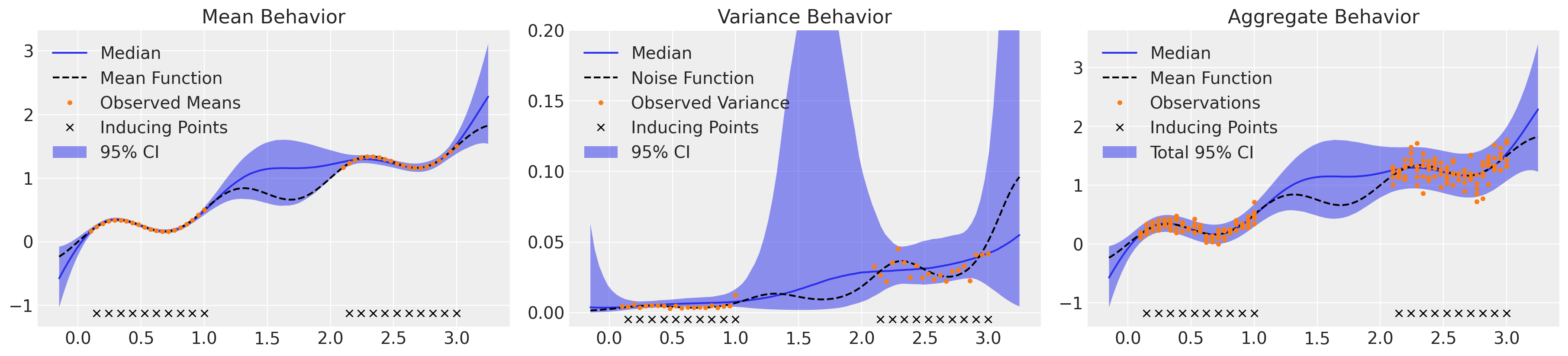
_, axs = plt.subplots(1, 3, figsize=(18, 4))
μ_samples = samples_hts["μ_pred"]
σ_samples = np.exp(samples_hts["lg_σ_pred"])
plot_mean(axs[0], μ_samples)
plot_inducing_points(axs[0])
plot_var(axs[1], σ_samples**2)
plot_inducing_points(axs[1])
plot_total(axs[2], μ_samples, σ_samples**2)
plot_inducing_points(axs[2])
那比原来快了约8倍,结果几乎无法区分,而且分歧也更少。
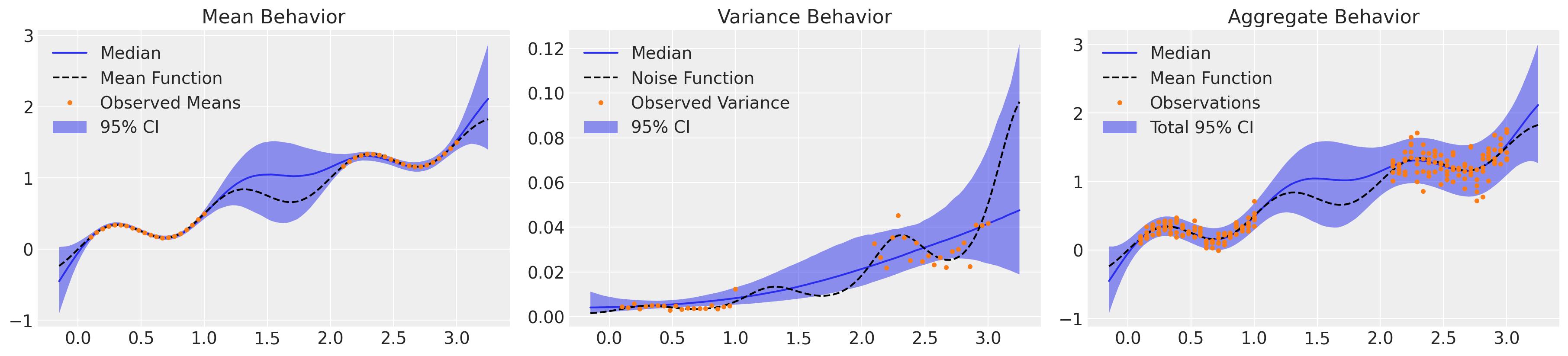
具有相关噪声和均值响应的异方差GP:协区域化线性模型#
到目前为止,我们已经将系统的均值和噪声建模为独立的。然而,在某些情况下,我们可能期望它们是相关的,例如,如果预期较高的测量值会有更大的噪声。在这里,我们将通过一个协方差函数显式地建模这种相关性,该协方差函数是我们之前使用的空间核与Coregion核的Kronecker积,正如Bill Engels在这里所建议的那样。这是线性区域化模型的实现,它将每个相关的GP视为少量独立基函数的线性组合,这些基函数本身也是GP。我们首先向观测域添加一个分类维度,以指示是考虑均值还是方差,然后在将它们输入如上所述的Normal似然之前解包各自的组件。
def add_coreg_idx(x):
    return np.hstack([np.tile(x, (2, 1)), np.vstack([np.zeros(x.shape), np.ones(x.shape)])])


Xu_c, X_obs_c, Xnew_c = [add_coreg_idx(x) for x in [Xu, X_obs, Xnew]]

with pm.Model() as model_htsc:
    ℓ = pm.InverseGamma("ℓ", mu=ℓ_μ, sigma=ℓ_σ)
    η = pm.Gamma("η", alpha=2, beta=1)
    EQcov = η**2 * pm.gp.cov.ExpQuad(input_dim=1, active_dims=[0], ls=ℓ)

    D_out = 2  # two output dimensions, mean and variance
    rank = 2  # two basis GPs
    W = pm.Normal("W", mu=0, sd=3, shape=(D_out, rank), testval=np.full([D_out, rank], 0.1))
    kappa = pm.Gamma("kappa", alpha=1.5, beta=1, shape=D_out)
    coreg = pm.gp.cov.Coregion(input_dim=1, active_dims=[0], kappa=kappa, W=W)

    cov = pm.gp.cov.Kron([EQcov, coreg])

    gp_LMC = SparseLatent(cov)
    LMC_f = gp_LMC.prior("LMC", X_obs_c, Xu_c)

    μ_f = LMC_f[: len(y_obs_)]
    lg_σ_f = LMC_f[len(y_obs_) :]
    σ_f = pm.Deterministic("σ_f", pm.math.exp(lg_σ_f))

    lik_htsc = pm.Normal("lik_htsc", mu=μ_f, sd=σ_f, observed=y_obs_)
    trace_htsc = pm.sample(target_accept=0.95, return_inferencedata=True, random_seed=SEED)

with model_htsc:
    c_mu_pred = gp_LMC.conditional("c_mu_pred", Xnew_c, Xu_c)
    samples_htsc = pm.sample_posterior_predictive(trace_htsc, var_names=["c_mu_pred"])
Auto-assigning NUTS sampler...
Initializing NUTS using jitter+adapt_diag...
Multiprocess sampling (4 chains in 4 jobs)
NUTS: [u_rotated_LMC, kappa, W, η, ℓ]
Sampling 4 chains for 1_000 tune and 1_000 draw iterations (4_000 + 4_000 draws total) took 8065 seconds.
There were 7 divergences after tuning. Increase `target_accept` or reparameterize.
There were 27 divergences after tuning. Increase `target_accept` or reparameterize.
There were 7 divergences after tuning. Increase `target_accept` or reparameterize.
There were 8 divergences after tuning. Increase `target_accept` or reparameterize.
The number of effective samples is smaller than 10% for some parameters.
μ_samples = samples_htsc["c_mu_pred"][:, : len(Xnew)]
σ_samples = np.exp(samples_htsc["c_mu_pred"][:, len(Xnew) :])

_, axs = plt.subplots(1, 3, figsize=(18, 4))
plot_mean(axs[0], μ_samples)
plot_inducing_points(axs[0])
plot_var(axs[1], σ_samples**2)
axs[1].set_ylim(-0.01, 0.2)
axs[1].legend(loc="upper left")
plot_inducing_points(axs[1])
plot_total(axs[2], μ_samples, σ_samples**2)
plot_inducing_points(axs[2])
我们可以通过检查通过 \(\mathbf{B} \equiv \mathbf{WW}^T+diag(\kappa)\) 构建的协方差矩阵 \(\bf{B}\) 来观察均值和方差之间的学习相关性:
with model_htsc:
    B_samples = pm.sample_posterior_predictive(trace_htsc, var_names=["W", "kappa"])
# Keep in mind that the first dimension in all arrays is the sampling dimension
W = B_samples["W"]
W_T = np.swapaxes(W, 1, 2)
WW_T = np.matmul(W, W_T)

kappa = B_samples["kappa"]
I = np.tile(np.identity(2), [kappa.shape[0], 1, 1])
# einsum is just a concise way of doing multiplication and summation over arbitrary axes
diag_kappa = np.einsum("ij,ijk->ijk", kappa, I)

B = WW_T + diag_kappa
B.mean(axis=0)
array([[15.72083568, -0.98047927],
       [-0.98047927, 11.53955904]])
sd = np.sqrt(np.diagonal(B, axis1=1, axis2=2))
outer_sd = np.einsum("ij,ik->ijk", sd, sd)
correlation = B / outer_sd
print(f"2.5%ile correlation: {np.percentile(correlation,2.5,axis=0)[0,1]:0.3f}")
print(f"Median correlation: {np.percentile(correlation,50,axis=0)[0,1]:0.3f}")
print(f"97.5%ile correlation: {np.percentile(correlation,97.5,axis=0)[0,1]:0.3f}")
2.5%ile correlation: -0.888
Median correlation: -0.086
97.5%ile correlation: 0.889
该模型无意中学习到均值和噪声略微负相关,尽管置信区间较宽。
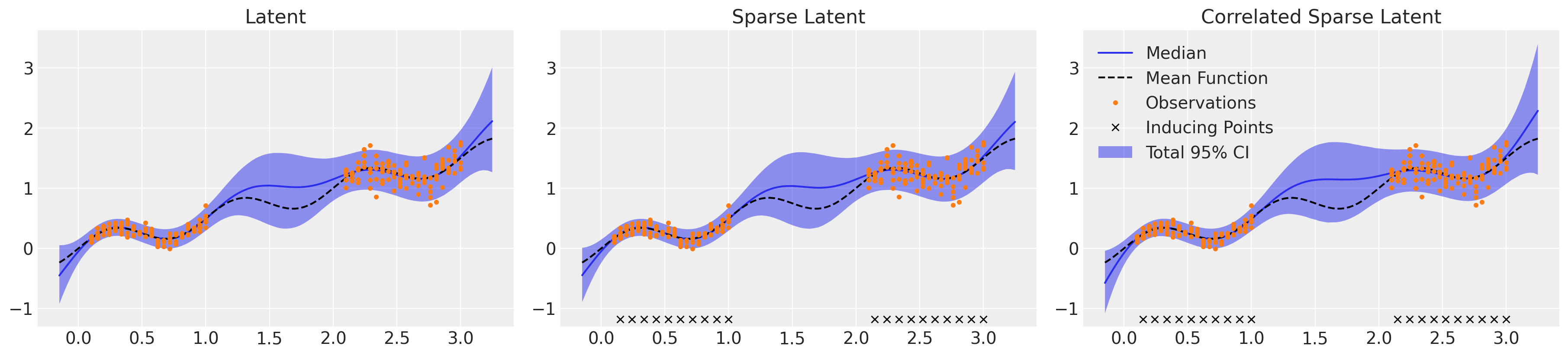
比较#
这里展示的三种潜在方法在复杂性和效率上有所不同,但最终产生了非常相似的回归曲面,如下所示。所有三种方法都展示了对于偶然不确定性和认知不确定性的细致理解。值得注意的是,我们不得不将target_accept从默认的0.8增加到0.95,以避免过多的分歧,但这有一个缺点,即减慢了NUTS评估的速度。采样时间可以通过减少target_accept来缩短,但代价是由于分歧可能导致推断偏差,或者通过进一步减少稀疏近似中使用的诱导点数量。检查每种方法的收敛统计数据,所有方法的r_hat值都较低,为1.01或以下,但LMC模型对某些参数的有效样本量较低,特别是η和ℓ参数的ess_tail。为了对该模型的95%置信区间边界有信心,我们应该运行更多的迭代采样,理想情况下至少直到最小的ess_tail超过200,但越高越好。
回归曲面#
_, axs = plt.subplots(1, 3, figsize=(18, 4))

μ_samples = samples_ht["μ_pred_ht"]
σ_samples = np.exp(samples_ht["lg_σ_pred_ht"])
plot_total(axs[0], μ_samples, σ_samples**2)
axs[0].set_title("Latent")

μ_samples = samples_hts["μ_pred"]
σ_samples = np.exp(samples_hts["lg_σ_pred"])
plot_total(axs[1], μ_samples, σ_samples**2)
axs[1].set_title("Sparse Latent")

μ_samples = samples_htsc["c_mu_pred"][:, : len(Xnew)]
σ_samples = np.exp(samples_htsc["c_mu_pred"][:, len(Xnew) :])
plot_total(axs[2], μ_samples, σ_samples**2)
axs[2].set_title("Correlated Sparse Latent")

yls = [ax.get_ylim() for ax in axs]
yl = [np.min([l[0] for l in yls]), np.max([l[1] for l in yls])]
for ax in axs:
    ax.set_ylim(yl)

plot_inducing_points(axs[1])
plot_inducing_points(axs[2])

axs[0].legend().remove()
axs[1].legend().remove()
潜在模型收敛#
display(az.summary(trace_ht).sort_values("ess_bulk").iloc[:5])
| mean | sd | hdi_3% | hdi_97% | mcse_mean | mcse_sd | ess_bulk | ess_tail | r_hat | |
|---|---|---|---|---|---|---|---|---|---|
| η | 1.886 | 0.731 | 0.749 | 3.311 | 0.028 | 0.020 | 659.0 | 812.0 | 1.0 |
| μ_f_rotated_[0] | 0.101 | 0.042 | 0.034 | 0.178 | 0.002 | 0.001 | 770.0 | 933.0 | 1.0 |
| ℓ | 0.581 | 0.061 | 0.472 | 0.700 | 0.002 | 0.001 | 920.0 | 846.0 | 1.0 |
| μ_f_rotated_[5] | 0.545 | 0.177 | 0.235 | 0.872 | 0.006 | 0.004 | 921.0 | 927.0 | 1.0 |
| σ_η | 1.939 | 0.748 | 0.882 | 3.303 | 0.020 | 0.014 | 1346.0 | 1176.0 | 1.0 |
稀疏潜在模型收敛#
display(az.summary(trace_hts).sort_values("ess_bulk").iloc[:5])
| mean | sd | hdi_3% | hdi_97% | mcse_mean | mcse_sd | ess_bulk | ess_tail | r_hat | |
|---|---|---|---|---|---|---|---|---|---|
| η | 1.857 | 0.681 | 0.777 | 3.183 | 0.022 | 0.016 | 850.0 | 1122.0 | 1.0 |
| u_rotated_μ[0] | 0.147 | 0.053 | 0.061 | 0.242 | 0.002 | 0.001 | 887.0 | 1276.0 | 1.0 |
| u_rotated_μ[1] | 0.345 | 0.110 | 0.157 | 0.548 | 0.004 | 0.003 | 929.0 | 1447.0 | 1.0 |
| u_rotated_μ[2] | -1.019 | 0.312 | -1.606 | -0.463 | 0.009 | 0.006 | 1232.0 | 1866.0 | 1.0 |
| u_rotated_μ[10] | 0.984 | 0.400 | 0.191 | 1.684 | 0.011 | 0.008 | 1264.0 | 2338.0 | 1.0 |