莫纳罗亚的二氧化碳高斯过程#

这个高斯过程（GP）示例展示了如何：

设计协方差函数的组合
使用加性高斯过程，其各个组成部分可用于预测
执行最大后验（MAP）估计

自20世纪50年代末以来，莫纳罗亚天文台一直在定期测量大气中的CO\(_2\)。在20世纪50年代末，查尔斯·基林发明了一种精确测量大气中CO\(_2\)浓度的方法。自那时起，CO\(_2\)的测量结果几乎连续不断地在莫纳罗亚天文台记录。查看最近一小时的测量结果这里。

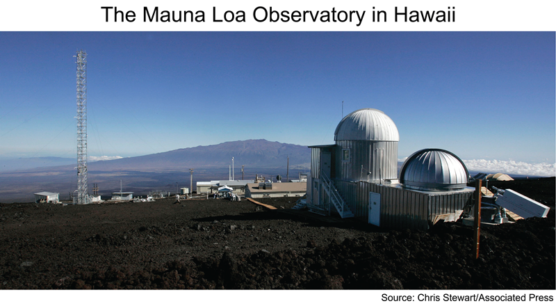
在20世纪50年代末，关于化石燃料燃烧如何影响气候的信息并不多。最初几年的数据收集显示，CO\(_2\)水平随着夏季和冬季的交替而上升和下降，这与北半球植被的生长和衰败相吻合。随着多年的过去，稳定上升的趋势越来越明显。在收集了超过70年的数据后，Keeling曲线成为了最重要的气候指标之一。

这些测量背后的历史及其对当今气候学的影响以及其他有趣的阅读：

http://scrippsco2.ucsd.edu/history_legacy/early_keeling_curve#
https://scripps.ucsd.edu/programs/keelingcurve/2016/05/23/为什么全球二氧化碳排放量的下降没有导致大气中二氧化碳水平的稳定/#more-1412

让我们加载数据，整理一下，然后看看。原始数据集位于此处。本笔记本使用Bokeh包来绘制受益于交互性的图表。

准备数据#

注意

本笔记本使用了不是 PyMC 依赖项的库，因此需要专门安装这些库才能运行此笔记本。打开下面的下拉菜单以获取更多指导。

import numpy as np
import pandas as pd
import pymc3 as pm

from bokeh.io import output_notebook
from bokeh.models import BoxAnnotation, Label, Legend, Span
from bokeh.palettes import brewer
from bokeh.plotting import figure, show

output_notebook()

Loading BokehJS ...

%config InlineBackend.figure_format = 'retina'
RANDOM_SEED = 8927
rng = np.random.default_rng(RANDOM_SEED)

# get data
try:
    data_monthly = pd.read_csv("../data/monthly_in_situ_co2_mlo.csv", header=56)
except FileNotFoundError:
    data_monthly = pd.read_csv(pm.get_data("monthly_in_situ_co2_mlo.csv"), header=56)

# replace -99.99 with NaN
data_monthly.replace(to_replace=-99.99, value=np.nan, inplace=True)

# fix column names
cols = [
    "year",
    "month",
    "--",
    "--",
    "CO2",
    "seasonaly_adjusted",
    "fit",
    "seasonally_adjusted_fit",
    "CO2_filled",
    "seasonally_adjusted_filled",
]
data_monthly.columns = cols
cols.remove("--")
cols.remove("--")
data_monthly = data_monthly[cols]

# drop rows with nan
data_monthly.dropna(inplace=True)

# fix time index
data_monthly["day"] = 15
data_monthly.index = pd.to_datetime(data_monthly[["year", "month", "day"]])
cols.remove("year")
cols.remove("month")
data_monthly = data_monthly[cols]

data_monthly.head(5)

	CO2	seasonaly_adjusted	fit	seasonally_adjusted_fit	CO2_filled	seasonally_adjusted_filled
1958-03-15	315.71	314.44	316.19	314.91	315.71	314.44
1958-04-15	317.45	315.16	317.30	314.99	317.45	315.16
1958-05-15	317.51	314.70	317.87	315.07	317.51	314.70
1958-07-15	315.86	315.20	315.86	315.22	315.86	315.20
1958-08-15	314.93	316.20	313.98	315.29	314.93	316.20

# function to convert datetimes to indexed numbers that are useful for later prediction
def dates_to_idx(timelist):
    reference_time = pd.to_datetime("1958-03-15")
    t = (timelist - reference_time) / pd.Timedelta(365, "D")
    return np.asarray(t)


t = dates_to_idx(data_monthly.index)

# normalize CO2 levels
y = data_monthly["CO2"].values
first_co2 = y[0]
std_co2 = np.std(y)
y_n = (y - first_co2) / std_co2

data_monthly = data_monthly.assign(t=t)
data_monthly = data_monthly.assign(y_n=y_n)

这些数据可能对你来说很熟悉，因为它被用作《机器学习中的高斯过程》一书中的示例，作者是 Rasmussen 和 Williams [2006]。他们使用的数据集版本始于20世纪50年代末，但截至2003年底。为了让我们的PyMC3示例与他们的示例具有一定的可比性，我们使用2004年之前的数据作为“训练”集。2004年至2022年的数据我们将用来测试我们的预测。

# split into training and test set
sep_idx = data_monthly.index.searchsorted(pd.to_datetime("2003-12-15"))
data_early = data_monthly.iloc[: sep_idx + 1, :]
data_later = data_monthly.iloc[sep_idx:, :]

# plot training and test data
p = figure(
    x_axis_type="datetime",
    title="Monthly CO2 Readings from Mauna Loa",
    plot_width=550,
    plot_height=350,
)
p.yaxis.axis_label = "CO2 [ppm]"
p.xaxis.axis_label = "Date"
predict_region = BoxAnnotation(
    left=pd.to_datetime("2003-12-15"), fill_alpha=0.1, fill_color="firebrick"
)
p.add_layout(predict_region)
ppm400 = Span(location=400, dimension="width", line_color="red", line_dash="dashed", line_width=2)
p.add_layout(ppm400)

p.line(data_monthly.index, data_monthly["CO2"], line_width=2, line_color="black", alpha=0.5)
p.circle(data_monthly.index, data_monthly["CO2"], line_color="black", alpha=0.1, size=2)

train_label = Label(
    x=100,
    y=165,
    x_units="screen",
    y_units="screen",
    text="Training Set",
    render_mode="css",
    border_line_alpha=0.0,
    background_fill_alpha=0.0,
)
test_label = Label(
    x=585,
    y=80,
    x_units="screen",
    y_units="screen",
    text="Test Set",
    render_mode="css",
    border_line_alpha=0.0,
    background_fill_alpha=0.0,
)

p.add_layout(train_label)
p.add_layout(test_label)
show(p)

Bokeh 图表是交互式的，因此可以通过右侧边栏进行平移和缩放。季节性的上升和下降非常明显，上升趋势也是如此。这里有一个链接，指向不同时间尺度下的此曲线的图表，以及在历史冰芯数据背景下的图表。

400 ppm 水平用虚线标出。除了拟合一个描述性模型外，我们的目标将是预测首次超过 400 ppm 阈值的月份，该月份是 2013年5月。在上面的数据集中，2013年5月的 CO\(_2\) 平均读数约为 399.98，接近我们的正确目标日期。

使用GPs建模Keeling曲线#

作为起点，我们使用了Rasmussen 和 Williams [2006]中描述的GP模型。与教科书中使用协方差函数超参数的平坦先验然后最大化边际似然不同，我们对超参数放置了稍微有信息的先验，并使用优化来找到MAP点。我们使用gp.Marginal，因为假设了高斯噪声。

R&W [Rasmussen 和 Williams, 2006] 模型是信号的三个GP之和，以及噪声的一个GP。

一个由指数二次核函数表示的长期平滑上升趋势。
一个周期性项，随着远离精确周期性而衰减。这由一个周期性和一个Matern52协方差函数的乘积表示。
具有有理二次核的小型和中型非周期性异常。
噪声被建模为Matern32和一个白噪声核的总和。

CO\(_2\)随时间变化的前验概率是，

\[ f(t) \sim \mathcal{GP}_{\text{slow}}(0,\, k_1(t, t')) + \mathcal{GP}_{\text{med}}(0,\, k_2(t, t')) + \mathcal{GP}_{\text{per}}(0,\, k_3(t, t')) + \mathcal{GP}_{\text{noise}}(0,\, k_4(t, t')) \]

超参数先验#

我们对协方差函数的尺度超参数使用相当不具信息的先验，对长度尺度使用信息丰富的Gamma参数。用于长度尺度先验的概率密度函数如下所示：

x = np.linspace(0, 150, 5000)
priors = [
    ("ℓ_pdecay", pm.Gamma.dist(alpha=10, beta=0.075)),
    ("ℓ_psmooth", pm.Gamma.dist(alpha=4, beta=3)),
    ("period", pm.Normal.dist(mu=1.0, sigma=0.05)),
    ("ℓ_med", pm.Gamma.dist(alpha=2, beta=0.75)),
    ("α", pm.Gamma.dist(alpha=5, beta=2)),
    ("ℓ_trend", pm.Gamma.dist(alpha=4, beta=0.1)),
    ("ℓ_noise", pm.Gamma.dist(alpha=2, beta=4)),
]

colors = brewer["Paired"][7]

p = figure(
    title="Lengthscale and period priors",
    plot_width=550,
    plot_height=350,
    x_range=(-1, 8),
    y_range=(0, 2),
)
p.yaxis.axis_label = "Probability"
p.xaxis.axis_label = "Years"

for i, prior in enumerate(priors):
    p.line(
        x,
        np.exp(prior[1].logp(x).eval()),
        legend_label=prior[0],
        line_width=3,
        line_color=colors[i],
    )
show(p)

ℓ_pdecay: 周期性衰减。这个参数越小，周期性消失得越快。我怀疑CO\(_2\)的季节性在不久的将来会消失（希望不会），而且数据中也没有证据表明这一点。大部分先验质量来自60到超过140年。
ℓ_psmooth: 周期性成分的平滑度。它控制周期性有多“正弦”。数据的图表显示季节性并不是一个精确的正弦波，但它与正弦波并没有太大的不同。我们使用一个模式在1的Gamma分布，并且方差不太大，大部分先验质量在0.5到2之间。
period: 周期。我们对\(p\)，即以1为中心的周期，设定了非常强的先验。R&W将\(p=1\)固定，因为周期是年度。
ℓ_med: 这是用于短至中等长期变化的长度尺度。这个先验分布的大部分质量在6年以下。
α: 这是形状参数。这个先验分布以3为中心，因为我们预计会有一些超出指数二次项解释范围的变化。
ℓ_trend: 长期趋势的长度尺度。它具有广泛的先验分布，主要集中在十年尺度上。大部分质量分布在10到60年之间。
ℓ_noise: 噪声协方差的长度尺度。这种噪声应该非常迅速，在几个月到最多一两年的尺度上。

我们事先知道哪些GP分量应该具有较大的幅度，因此我们将此信息包含在尺度参数中。

x = np.linspace(0, 4, 5000)
priors = [
    ("η_per", pm.HalfCauchy.dist(beta=2)),
    ("η_med", pm.HalfCauchy.dist(beta=1.0)),
    (
        "η_trend",
        pm.HalfCauchy.dist(beta=3),
    ),  # will use beta=2, but beta=3 is visible on plot
    ("σ", pm.HalfNormal.dist(sigma=0.25)),
    ("η_noise", pm.HalfNormal.dist(sigma=0.5)),
]

colors = brewer["Paired"][5]

p = figure(title="Scale priors", plot_width=550, plot_height=350)
p.yaxis.axis_label = "Probability"
p.xaxis.axis_label = "Years"

for i, prior in enumerate(priors):
    p.line(
        x,
        np.exp(prior[1].logp(x).eval()),
        legend_label=prior[0],
        line_width=3,
        line_color=colors[i],
    )
show(p)

对于所有的尺度先验，我们使用将尺度向零收缩的分布。季节性成分和长期趋势在零附近的质量最少，因为它们是对数据影响最大的因素。

η_per: 周期性或季节性成分的尺度。
η_med: 短期到中期成分的尺度。
η_trend: 长期趋势的尺度。
σ: 白噪声的尺度。
η_noise: 相关短期噪声的尺度。

PyMC3 中的模型#

下面是实际的模型。三个组件中的每一个高斯过程（GP）都是单独构建的。由于我们正在进行最大后验概率（MAP），我们使用边际高斯过程，最后调用.marginal_likelihood方法来指定边际后验。

# pull out normalized data
t = data_early["t"].values[:, None]
y = data_early["y_n"].values

with pm.Model() as model:
    # yearly periodic component x long term trend
    η_per = pm.HalfCauchy("η_per", beta=2, testval=1.0)
    ℓ_pdecay = pm.Gamma("ℓ_pdecay", alpha=10, beta=0.075)
    period = pm.Normal("period", mu=1, sigma=0.05)
    ℓ_psmooth = pm.Gamma("ℓ_psmooth ", alpha=4, beta=3)
    cov_seasonal = (
        η_per**2 * pm.gp.cov.Periodic(1, period, ℓ_psmooth) * pm.gp.cov.Matern52(1, ℓ_pdecay)
    )
    gp_seasonal = pm.gp.Marginal(cov_func=cov_seasonal)

    # small/medium term irregularities
    η_med = pm.HalfCauchy("η_med", beta=0.5, testval=0.1)
    ℓ_med = pm.Gamma("ℓ_med", alpha=2, beta=0.75)
    α = pm.Gamma("α", alpha=5, beta=2)
    cov_medium = η_med**2 * pm.gp.cov.RatQuad(1, ℓ_med, α)
    gp_medium = pm.gp.Marginal(cov_func=cov_medium)

    # long term trend
    η_trend = pm.HalfCauchy("η_trend", beta=2, testval=2.0)
    ℓ_trend = pm.Gamma("ℓ_trend", alpha=4, beta=0.1)
    cov_trend = η_trend**2 * pm.gp.cov.ExpQuad(1, ℓ_trend)
    gp_trend = pm.gp.Marginal(cov_func=cov_trend)

    # noise model
    η_noise = pm.HalfNormal("η_noise", sigma=0.5, testval=0.05)
    ℓ_noise = pm.Gamma("ℓ_noise", alpha=2, beta=4)
    σ = pm.HalfNormal("σ", sigma=0.25, testval=0.05)
    cov_noise = η_noise**2 * pm.gp.cov.Matern32(1, ℓ_noise) + pm.gp.cov.WhiteNoise(σ)

    # The Gaussian process is a sum of these three components
    gp = gp_seasonal + gp_medium + gp_trend

    # Since the normal noise model and the GP are conjugates, we use `Marginal` with the `.marginal_likelihood` method
    y_ = gp.marginal_likelihood("y", X=t, y=y, noise=cov_noise)

    # this line calls an optimizer to find the MAP
    mp = pm.find_MAP(include_transformed=True)

100.00% [300/300 00:52<00:00 logp = 1,734.4, ||grad|| = 14.264]

# display the results, dont show transformed parameter values
sorted([name + ":" + str(mp[name]) for name in mp.keys() if not name.endswith("_")])

['period:1.00038447904791',
 'α:1.1815982319316372',
 'η_med:0.021391276520692636',
 'η_noise:0.006819703084865676',
 'η_per:0.08803544888083512',
 'η_trend:1.712437847900024',
 'σ:0.0059989944162813155',
 'ℓ_med:1.507055362902511',
 'ℓ_noise:0.16455363060019101',
 'ℓ_pdecay:125.58803198611457',
 'ℓ_psmooth :0.7229240021307682',
 'ℓ_trend:52.58970494079544']

乍一看，结果看起来是合理的。决定季节性变化速度的长度尺度约为126年。这意味着，根据数据，我们预计这种强烈的周期性不会消失，直到几个世纪过去。趋势长度尺度也很长，大约50年。

检查每个加性GP分量的拟合情况#

下面的代码检查了总GP的拟合情况，以及每个组件的单独拟合情况。总拟合及其\(2\sigma\)不确定性以红色显示。

# predict at a 15 day granularity
dates = pd.date_range(start="3/15/1958", end="12/15/2003", freq="15D")
tnew = dates_to_idx(dates)[:, None]

print("Predicting with gp ...")
mu, var = gp.predict(tnew, point=mp, diag=True)
mean_pred = mu * std_co2 + first_co2
var_pred = var * std_co2**2

# make dataframe to store fit results
fit = pd.DataFrame(
    {"t": tnew.flatten(), "mu_total": mean_pred, "sd_total": np.sqrt(var_pred)},
    index=dates,
)

print("Predicting with gp_trend ...")
mu, var = gp_trend.predict(
    tnew, point=mp, given={"gp": gp, "X": t, "y": y, "noise": cov_noise}, diag=True
)
fit = fit.assign(mu_trend=mu * std_co2 + first_co2, sd_trend=np.sqrt(var * std_co2**2))

print("Predicting with gp_medium ...")
mu, var = gp_medium.predict(
    tnew, point=mp, given={"gp": gp, "X": t, "y": y, "noise": cov_noise}, diag=True
)
fit = fit.assign(mu_medium=mu * std_co2 + first_co2, sd_medium=np.sqrt(var * std_co2**2))

print("Predicting with gp_seasonal ...")
mu, var = gp_seasonal.predict(
    tnew, point=mp, given={"gp": gp, "X": t, "y": y, "noise": cov_noise}, diag=True
)
fit = fit.assign(mu_seasonal=mu * std_co2 + first_co2, sd_seasonal=np.sqrt(var * std_co2**2))
print("Done")

Predicting with gp ...
Predicting with gp_trend ...
Predicting with gp_medium ...
Predicting with gp_seasonal ...
Done

## plot the components
p = figure(
    title="Decomposition of the Mauna Loa Data",
    x_axis_type="datetime",
    plot_width=550,
    plot_height=350,
)
p.yaxis.axis_label = "CO2 [ppm]"
p.xaxis.axis_label = "Date"

# plot mean and 2σ region of total prediction
upper = fit.mu_total + 2 * fit.sd_total
lower = fit.mu_total - 2 * fit.sd_total
band_x = np.append(fit.index.values, fit.index.values[::-1])
band_y = np.append(lower, upper[::-1])

# total fit
p.line(
    fit.index,
    fit.mu_total,
    line_width=1,
    line_color="firebrick",
    legend_label="Total fit",
)
p.patch(band_x, band_y, color="firebrick", alpha=0.6, line_color="white")

# trend
p.line(
    fit.index,
    fit.mu_trend,
    line_width=1,
    line_color="blue",
    legend_label="Long term trend",
)

# medium
p.line(
    fit.index,
    fit.mu_medium,
    line_width=1,
    line_color="green",
    legend_label="Medium range variation",
)

# seasonal
p.line(
    fit.index,
    fit.mu_seasonal,
    line_width=1,
    line_color="orange",
    legend_label="Seasonal process",
)

# true value
p.circle(data_early.index, data_early["CO2"], color="black", legend_label="Observed data")
p.legend.location = "top_left"
show(p)

拟合结果与观测数据非常吻合。趋势、季节性和短期/中期效应也清晰地分离出来。如果你放大到季节性过程填满绘图窗口（从x等于1955到2004，从y等于310到320），随着时间的推移，它似乎在逐渐变宽。让我们绘制每十年的第一年：

# plot several years

p = figure(title="Several years of the seasonal component", plot_width=550, plot_height=350)
p.yaxis.axis_label = "Δ CO2 [ppm]"
p.xaxis.axis_label = "Month"

colors = brewer["Paired"][5]
years = ["1960", "1970", "1980", "1990", "2000"]

for i, year in enumerate(years):
    dates = pd.date_range(start="1/1/" + year, end="12/31/" + year, freq="10D")
    tnew = dates_to_idx(dates)[:, None]

    print("Predicting year", year)
    mu, var = gp_seasonal.predict(
        tnew, point=mp, diag=True, given={"gp": gp, "X": t, "y": y, "noise": cov_noise}
    )
    mu_pred = mu * std_co2

    # plot mean
    x = np.asarray((dates - dates[0]) / pd.Timedelta(30, "D")) + 1
    p.line(x, mu_pred, line_width=1, line_color=colors[i], legend_label=year)

p.legend.location = "bottom_left"
show(p)

Predicting year 1960
Predicting year 1970
Predicting year 1980
Predicting year 1990
Predicting year 2000

这个图表清楚地表明，随着时间的推移，情况有所扩大。因此，似乎随着大气中CO\(_2\)的增加，由于北半球植被的生长和衰败导致的吸收/释放周期变得更加明显。

二氧化碳水平何时会突破400 ppm？#

我们的预测看起来如何？显然，观察到的数据呈上升趋势，季节性效应非常明显。我们的GP模型是否能够很好地捕捉这一点，从而做出合理的推断？我们的“训练”集一直持续到2003年底，因此我们将从2004年1月开始预测，直到2022年底。

尽管这一事件除了是一个不错的整数外没有特别的意义，我们的次要目标是看看我们能多好地预测首次达到400 ppm标记的日期。这一事件首次发生在2013年5月，并且有几篇关于其他重要里程碑的新闻文章。

dates = pd.date_range(start="11/15/2003", end="12/15/2022", freq="10D")
tnew = dates_to_idx(dates)[:, None]

print("Sampling gp predictions ...")
mu_pred, cov_pred = gp.predict(tnew, point=mp)

# draw samples, and rescale
n_samples = 2000
samples = pm.MvNormal.dist(mu=mu_pred, cov=cov_pred, shape=(n_samples, len(tnew))).random()
samples = samples * std_co2 + first_co2

Sampling gp predictions ...

# make plot
p = figure(x_axis_type="datetime", plot_width=700, plot_height=300)
p.yaxis.axis_label = "CO2 [ppm]"
p.xaxis.axis_label = "Date"

# plot mean and 2σ region of total prediction
# scale mean and var
mu_pred_sc = mu_pred * std_co2 + first_co2
sd_pred_sc = np.sqrt(np.diag(cov_pred) * std_co2**2)

upper = mu_pred_sc + 2 * sd_pred_sc
lower = mu_pred_sc - 2 * sd_pred_sc
band_x = np.append(dates, dates[::-1])
band_y = np.append(lower, upper[::-1])

p.line(dates, mu_pred_sc, line_width=2, line_color="firebrick", legend_label="Total fit")
p.patch(band_x, band_y, color="firebrick", alpha=0.6, line_color="white")

# some predictions
idx = np.random.randint(0, samples.shape[0], 10)
p.multi_line(
    [dates] * len(idx),
    [samples[i, :] for i in idx],
    color="firebrick",
    alpha=0.5,
    line_width=0.5,
)

# true value
p.circle(data_later.index, data_later["CO2"], color="black", legend_label="Observed data")

ppm400 = Span(
    location=400,
    dimension="width",
    line_color="black",
    line_dash="dashed",
    line_width=1,
)
p.add_layout(ppm400)
p.legend.location = "bottom_right"
show(p)

平均预测值和\(2\sigma\)不确定性以红色显示。还显示了边缘后验分布的几个样本。看起来我们的模型对二氧化碳释放量的估计有些乐观。\(2\sigma\)不确定性首次超过400 ppm阈值的时间是2015年5月，比预期晚了两年。

发生这种情况的一个原因是我们的GP先验具有零均值。这意味着我们编码了先验信息，表明随着我们远离观测数据，函数应该趋近于零。这个假设可能是不合理的。也有可能是CO\(_2\)趋势的增长速度比线性增长更快——这对于准确预测非常重要。另一个可能性是MAP估计。如果不查看完整的后验分布，我们对估计的不确定性会被低估。具体低估的程度是未知的。

具有零均值的GP先验导致预测结果偏差较大。解决此问题的一些可能性是使用一个常数均值函数，其值可能被赋值为历史或工业革命前的CO\(_2\)平均值。然而，这可能不是未来CO\(_2\)水平的最佳指标。

此外，仅使用历史CO\(_2\)数据可能不是最佳预测方法。除了通过GP拟合来观察决定CO\(_2\)水平的潜在行为外，我们还可以结合其他信息，例如化石燃料燃烧释放的CO\(_2\)量。

接下来，我们将了解如何使用 PyMC3 的 GP 功能来改进模型，查看完整的后验分布，并结合其他关于 CO\(_2\) 水平驱动因素的数据。

作者#

由Bill Engels于2017年9月撰写（pymc#2444）
由 Chris Fonnesbeck 于 2020 年 12 月更新
由Danh Phan于2022年5月重新执行（pymc-examples#316）

参考资料#

[1] (1,2,3)

卡尔·爱德华·拉斯穆森和克里斯托弗·K.I.威廉姆斯。《高斯过程在机器学习中的应用》。麻省理工学院出版社，2006年。ISBN 026218253X。网址：https://gaussianprocess.org/gpml/。

%load_ext watermark
%watermark -n -u -v -iv -w -p bokeh

Last updated: Fri May 06 2022

Python implementation: CPython
Python version       : 3.9.5
IPython version      : 7.25.0

bokeh: 2.4.2

numpy : 1.21.0
pandas: 1.4.0
pymc3 : 3.11.4

Watermark: 2.3.0

许可证声明#

本示例库中的所有笔记本均在MIT许可证下提供，该许可证允许修改和重新分发，前提是保留版权和许可证声明。

引用 PyMC 示例#

要引用此笔记本，请使用Zenodo为pymc-examples仓库提供的DOI。

重要

许多笔记本是从其他来源改编的：博客、书籍……在这种情况下，您应该引用原始来源。

同时记得引用代码中使用的相关库。

这是一个BibTeX的引用模板：

@incollection{citekey,
  author    = "<notebook authors, see above>",
  title     = "<notebook title>",
  editor    = "PyMC Team",
  booktitle = "PyMC examples",
  doi       = "10.5281/zenodo.5654871"
}

渲染后可能看起来像：

分类

标签