示例：Mauna Loa CO\(_2\) 继续

这个GP示例展示了如何

• 使用NUTS拟合完全贝叶斯GP

• 模型输入，其确切位置不确定（‘x’中的不确定性）

• 设计一个半参数高斯过程模型

• 构建一个变化点协方差函数/核

• 定义一个自定义的均值和自定义的协方差函数

冰芯数据

我们将查看的第一个数据集是来自冰芯数据的二氧化碳测量值。这些数据可以追溯到公元13年。1958年之后的数据是冰芯测量值和从莫纳罗亚山获取的更准确数据的平均值。我非常感谢来自伯尔尼大学的Tobias Erhardt，他慷慨地分享了关于一些实际涉及的过程如何工作的科学见解。当然，任何错误都是我自己的。

这些数据不如莫纳罗亚大气CO2测量值准确。落在南极洲的雪逐渐积累并随着时间的推移硬化成冰，这被称为粒雪。劳德冰芯中测量的CO2来自冰中被困的气泡。如果这些冰是瞬间冻结的，气泡中含有的CO2量将反映冻结时大气中CO2的确切量。然而，这个过程是逐渐发生的，所以被困的空气有时间在整个固化的冰中扩散。粒雪的分层、冻结和固化过程发生在数年的时间尺度上。对于这里使用的劳德冰芯数据，数据中列出的CO2测量值代表了大约2-4年内的平均CO2值。

此外，数据点的顺序是固定的。旧的冰层不可能出现在新的冰层之上。这要求我们对测量位置施加一个顺序受限的先验。

冰芯测量的日期存在一定的不确定性。由于冰层每年都会形成，因此年份级别的准确性可能是准确的，但测量时的季节性日期不太可能可靠。此外，观察到的二氧化碳水平可能是全年总体水平的某种平均值。

正如我们在前面的例子中看到的，二氧化碳水平中存在一个强烈的季节性成分，这在当前的数据集中是不可观察的。在 PyMC3 中，我们可以轻松地包含 \(y\) 和 \(x\) 中的误差。为了演示这一点，我们移除了数据的后半部分（这部分数据与莫纳罗亚的读数进行了平均），因此我们只有冰芯测量数据。我们使用 No-U-Turn MCMC 采样器来拟合高斯过程模型。

import arviz as az
import matplotlib.pyplot as plt
import numpy as np
import pandas as pd
import pymc3 as pm
import theano
import theano.tensor as tt

%config InlineBackend.figure_format = 'retina'
RANDOM_SEED = 8927
np.random.seed(RANDOM_SEED)
az.style.use("arviz-darkgrid")

ice = pd.read_csv(pm.get_data("merged_ice_core_yearly.csv"), header=26)
ice.columns = ["year", "CO2"]
ice["CO2"] = ice["CO2"].astype(np.float)

#### DATA AFTER 1958 is an average of ice core and mauna loa data, so remove it
ice = ice[ice["year"] <= 1958]
print("Number of data points:", len(ice))

Number of data points: 111

fig = plt.figure(figsize=(9, 4))
ax = plt.gca()

ax.plot(ice.year.values, ice.CO2.values, ".k")
ax.set_xlabel("Year")
ax.set_ylabel("CO2 (ppm)");

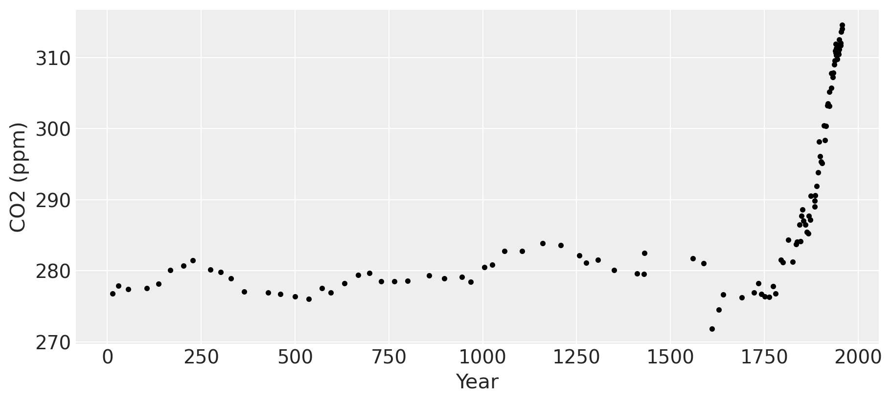
工业革命时期大约发生在1760年至1840年之间。这一点在图中清晰可见，二氧化碳水平在长期稳定在约280 ppm后急剧上升。

‘x’中的不确定性

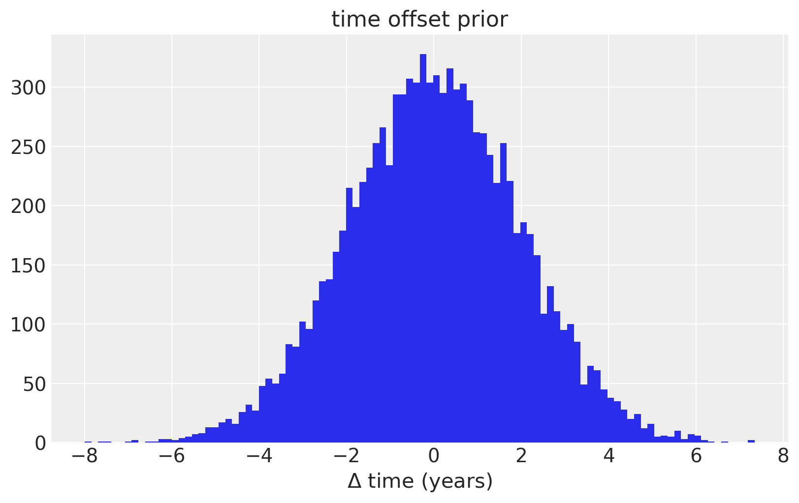
为了对\(x\)或时间中的不确定性进行建模，我们在每个观测日期上放置了一个先验分布。为了使先验标准化，我们特别使用了一个PyMC3随机变量来建模数据集中给定日期与其误差之间的差异。我们假设这些差异是均值为零、标准差为两年的正态分布。我们还通过使用ordered变换来确保观测值在时间上有严格的顺序。

对于仅冰芯数据而言，\(x\) 的不确定性并不是非常重要。在最后一个示例中，我们将看到它在模型中如何发挥更重要的作用。

fig = plt.figure(figsize=(8, 5))
ax = plt.gca()
ax.hist(100 * pm.Normal.dist(mu=0.0, sigma=0.02).random(size=10000), 100)
ax.set_xlabel(r"$\Delta$ time (years)")
ax.set_title("time offset prior");

t = ice.year.values
y = ice.CO2.values

# normalize the CO2 readings prior to fitting the model
y_mu, y_sd = np.mean(y[0:50]), np.std(y)
y_n = (y - y_mu) / y_sd

# scale t to have units of centuries
t_n = t / 100

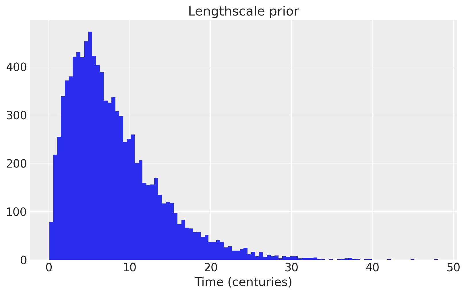
我们使用了一个信息先验在长度尺度上，将大部分质量分布在几个到20个世纪之间。

fig = plt.figure(figsize=(8, 5))
ax = plt.gca()
ax.hist(pm.Gamma.dist(alpha=2, beta=0.25).random(size=10000), 100)
ax.set_xlabel("Time (centuries)")
ax.set_title("Lengthscale prior");

with pm.Model() as model:
    η = pm.HalfNormal("η", sigma=5)
    ℓ = pm.Gamma("ℓ", alpha=4, beta=2)
    α = pm.Gamma("α", alpha=3, beta=1)
    cov = η**2 * pm.gp.cov.RatQuad(1, α, ℓ)

    gp = pm.gp.Marginal(cov_func=cov)

    # x location uncertainty
    # - sd = 0.02 says the uncertainty on the point is about two years
    t_diff = pm.Normal("t_diff", mu=0.0, sigma=0.02, shape=len(t))
    t_uncert = t_n - t_diff

    # white noise variance
    σ = pm.HalfNormal("σ", sigma=5, testval=1)
    y_ = gp.marginal_likelihood("y", X=t_uncert[:, None], y=y_n, noise=σ)

/Users/alex_andorra/tptm_alex/pymc3/pymc3/gp/cov.py:93: UserWarning: Only 1 column(s) out of Subtensor{int64}.0 are being used to compute the covariance function. If this is not intended, increase 'input_dim' parameter to the number of columns to use. Ignore otherwise.
  " the number of columns to use. Ignore otherwise.", UserWarning)

接下来我们可以使用NUTS MCMC算法进行采样。我们运行两个链，但将核心数设置为一个，因为Theano内部使用的线性代数库是多核的。

with model:
    tr = pm.sample(target_accept=0.95, return_inferencedata=True)

Auto-assigning NUTS sampler...
Initializing NUTS using jitter+adapt_diag...
Multiprocess sampling (4 chains in 4 jobs)
NUTS: [σ, t_diff, α, ℓ, η]

100.00% [8000/8000 02:07<00:00 Sampling 4 chains, 0 divergences]

Sampling 4 chains for 1_000 tune and 1_000 draw iterations (4_000 + 4_000 draws total) took 136 seconds.

az.plot_trace(tr, var_names=["t_diff"], compact=True);

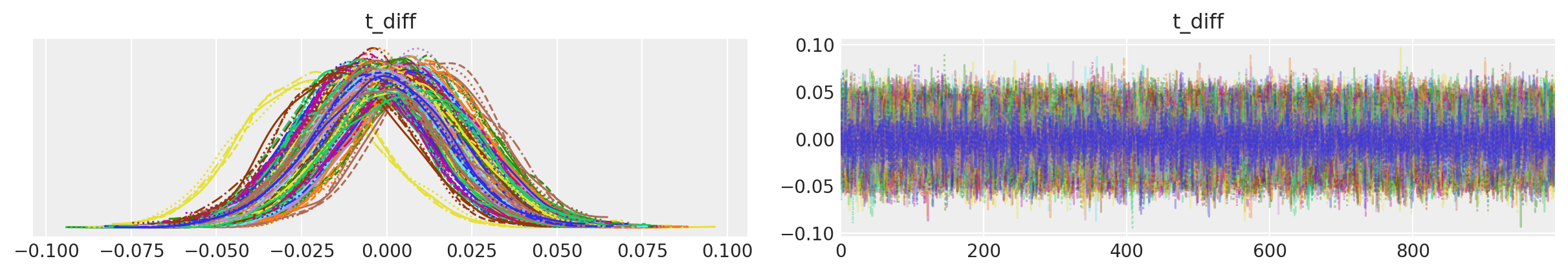
在t_diff的轨迹图中，我们可以看到不同输入的后验峰值没有移动太多，但位置的不确定性通过采样得到了考虑。

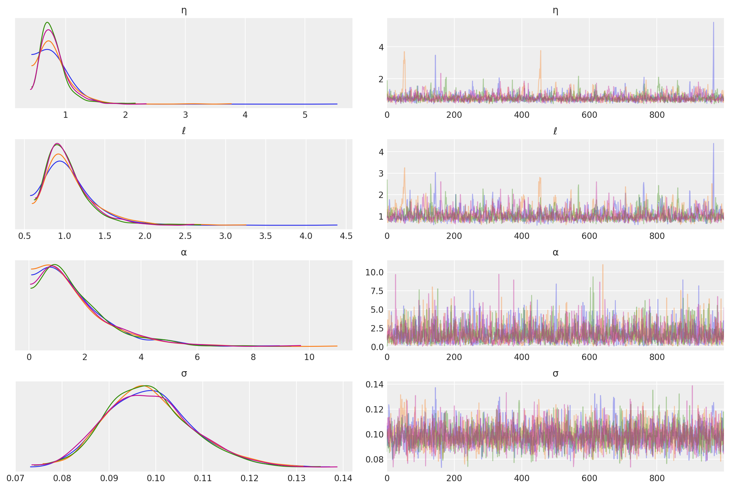
其他未知超参数的后验分布如下。

az.plot_trace(tr, var_names=["η", "ℓ", "α", "σ"]);

预测

tnew = np.linspace(-100, 2150, 2000) * 0.01
with model:
    fnew = gp.conditional("fnew", Xnew=tnew[:, None])

with model:
    ppc = pm.sample_posterior_predictive(tr, samples=100, var_names=["fnew"])

/Users/alex_andorra/tptm_alex/pymc3/pymc3/gp/cov.py:93: UserWarning: Only 1 column(s) out of Subtensor{int64}.0 are being used to compute the covariance function. If this is not intended, increase 'input_dim' parameter to the number of columns to use. Ignore otherwise.
  " the number of columns to use. Ignore otherwise.", UserWarning)
/Users/alex_andorra/tptm_alex/pymc3/pymc3/sampling.py:1708: UserWarning: samples parameter is smaller than nchains times ndraws, some draws and/or chains may not be represented in the returned posterior predictive sample
  "samples parameter is smaller than nchains times ndraws, some draws "

100.00% [100/100 09:05<00:00]

samples = y_sd * ppc["fnew"] + y_mu

fig = plt.figure(figsize=(12, 5))
ax = plt.gca()
pm.gp.util.plot_gp_dist(ax, samples, tnew * 100, plot_samples=True, palette="Blues")
ax.plot(t, y, "k.")
ax.set_xlim([-100, 2200])
ax.set_ylabel("CO2")
ax.set_xlabel("Year");

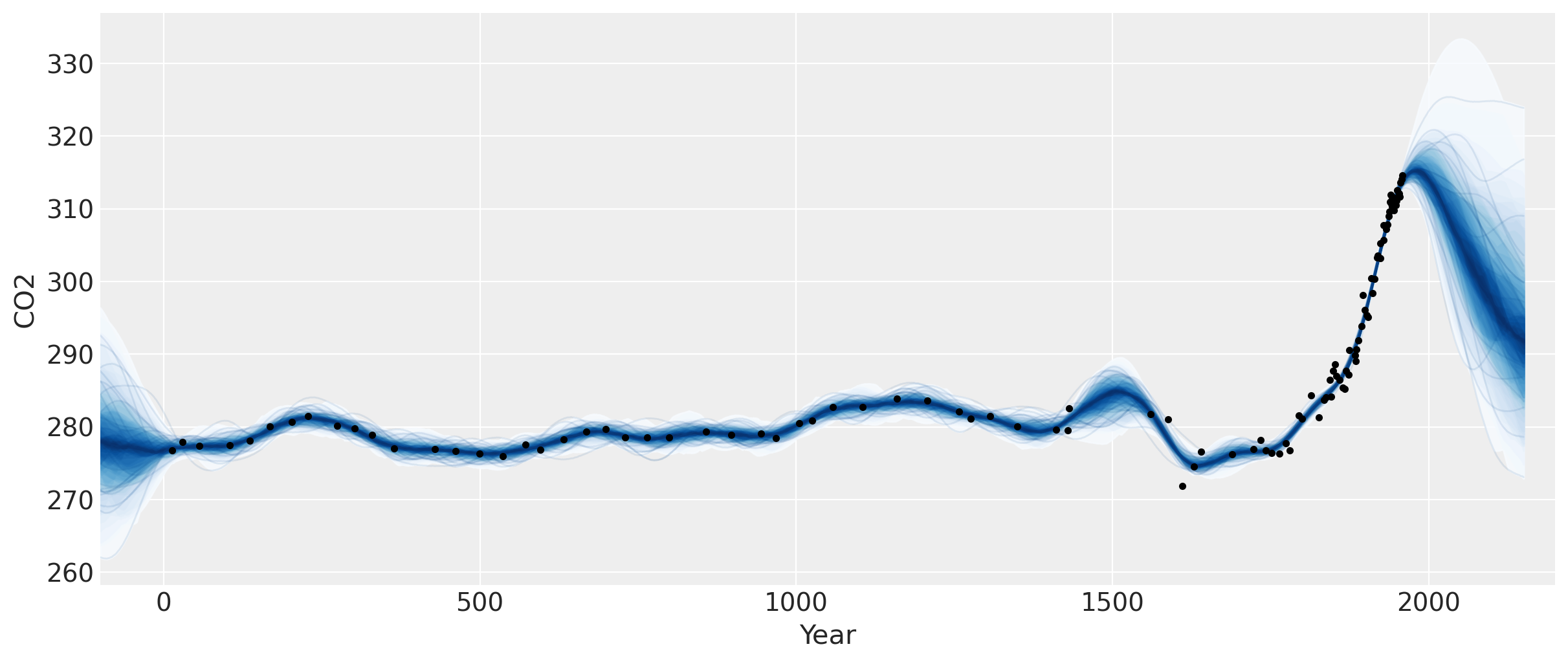
这个图中有两个明显的特征。一个是小冰期，其对二氧化碳的影响发生在1600年到1800年左右。另一个是工业革命，当时人们开始向大气中释放大量二氧化碳。

半参数高斯过程

在1958年最新数据点之后的预测显示上升，然后趋于平稳，接着再次下降。我们应该相信这个预测吗？我们知道它并没有得到验证（参见前一个笔记本），因为二氧化碳水平继续上升。

我们没有在我们的模型中指定均值函数，所以我们假设我们的高斯过程的均值为零。这意味着当我们对未来进行预测时，函数最终会回归到零。在这种情况下，这是否合理？目前没有任何全球性事件表明大气中的二氧化碳不会继续其当前的趋势。

用于变更点的线性模型

我们采用了Facebook的prophet时间序列模型所使用的公式。这是一个线性分段函数，其中每个段的端点被限制为相互连接。下面绘制了一些示例函数。

def dm_changepoints(t, changepoints_t):
    A = np.zeros((len(t), len(changepoints_t)))
    for i, t_i in enumerate(changepoints_t):
        A[t >= t_i, i] = 1
    return A

为了以后使用，我们使用符号化的theano变量重新编写了这个函数。代码有点难以理解，但它返回的结果与dm_changepoitns相同，同时避免了使用循环。

def dm_changepoints_theano(X, changepoints_t):
    return 0.5 * (1.0 + tt.sgn(tt.tile(X, (1, len(changepoints_t))) - changepoints_t))

从图中可以看出，一些可能的变点位置在1600年、1800年，也许还有1900年。这些时间点标志着小冰期的结束、工业革命的开始以及更现代工业实践的开始。

changepoints_t = np.array([16, 18, 19])

A = dm_changepoints(t_n, changepoints_t)

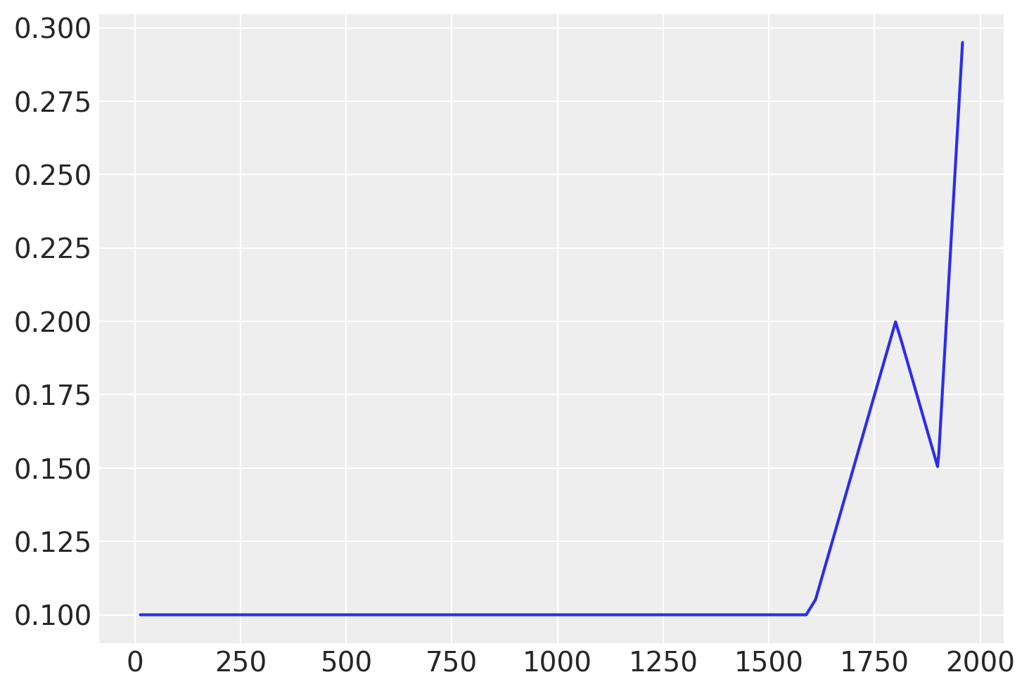
有几个参数（我们将进行估计），一些测试值和结果函数的图形如下所示

# base growth rate, or initial slope
k = 0.0

# offset
m = 0.1

# slope parameters
delta = np.array([0.05, -0.1, 0.3])

x = (k + np.dot(A, delta)) * t_n + (m + np.dot(A, -changepoints_t * delta))
plt.plot(t, x);

自定义变点均值函数

我们可以直接编码这个均值函数，但如果我们将其包装在一个Mean对象中，那么使用其他高斯过程功能会更方便，比如.conditional和.predict方法。请参阅自定义均值和协方差函数的更多信息。我们只需要定义__init__和__call__函数。

class PiecewiseLinear(pm.gp.mean.Mean):
    def __init__(self, changepoints, k, m, delta):
        self.changepoints = changepoints
        self.k = k
        self.m = m
        self.delta = delta

    def __call__(self, X):
        # X are the x locations, or time points
        A = dm_changepoints_theano(X, self.changepoints)
        return (self.k + tt.dot(A, self.delta)) * X.flatten() + (
            self.m + tt.dot(A, -self.changepoints * self.delta)
        )

每次评估均值函数时重新创建A是低效的，但当进行预测时输入的数量发生变化时，我们需要这样做。

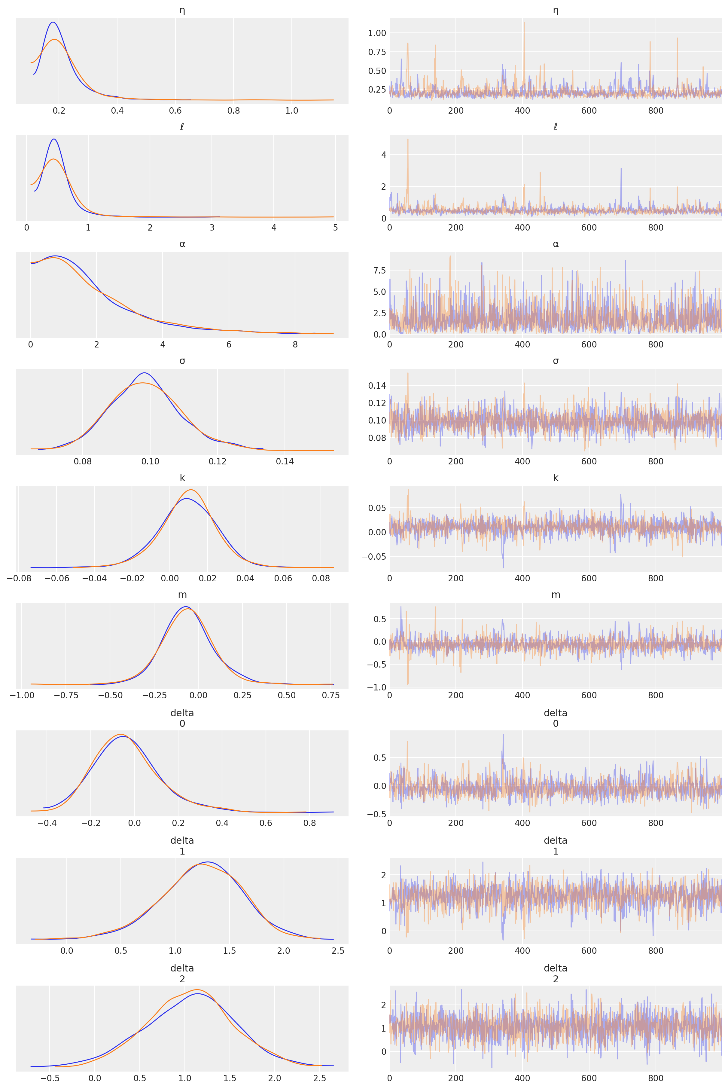
半参数变化点模型

接下来是更新后的模型，包含变化点的均值函数。

with pm.Model() as model:
    η = pm.HalfNormal("η", sigma=2)
    ℓ = pm.Gamma("ℓ", alpha=4, beta=2)
    α = pm.Gamma("α", alpha=3, beta=1)
    cov = η**2 * pm.gp.cov.RatQuad(1, α, ℓ)

    # piecewise linear mean function
    k = pm.Normal("k", mu=0, sigma=1)
    m = pm.Normal("m", mu=0, sigma=1)
    delta = pm.Normal("delta", mu=0, sigma=5, shape=len(changepoints_t))
    mean = PiecewiseLinear(changepoints_t, k, m, delta)

    # include mean function in GP constructor
    gp = pm.gp.Marginal(cov_func=cov, mean_func=mean)

    # x location uncertainty
    # - sd = 0.02 says the uncertainty on the point is about two years
    t_diff = pm.Normal("t_diff", mu=0.0, sigma=0.02, shape=len(t))
    t_uncert = t_n - t_diff

    # white noise variance
    σ = pm.HalfNormal("σ", sigma=5)
    y_ = gp.marginal_likelihood("y", X=t_uncert[:, None], y=y_n, noise=σ)

/Users/alex_andorra/tptm_alex/pymc3/pymc3/gp/cov.py:93: UserWarning: Only 1 column(s) out of Subtensor{int64}.0 are being used to compute the covariance function. If this is not intended, increase 'input_dim' parameter to the number of columns to use. Ignore otherwise.
  " the number of columns to use. Ignore otherwise.", UserWarning)

with model:
    tr = pm.sample(chains=2, target_accept=0.95)

Auto-assigning NUTS sampler...
Initializing NUTS using jitter+adapt_diag...
Multiprocess sampling (2 chains in 4 jobs)
NUTS: [σ, t_diff, delta, m, k, α, ℓ, η]

100.00% [4000/4000 03:22<00:00 Sampling 2 chains, 0 divergences]

Sampling 2 chains for 1_000 tune and 1_000 draw iterations (2_000 + 2_000 draws total) took 208 seconds.

az.plot_trace(tr, var_names=["η", "ℓ", "α", "σ", "k", "m", "delta"]);

/Users/alex_andorra/opt/anaconda3/envs/dev-pymc/lib/python3.6/site-packages/arviz/data/io_pymc3.py:89: FutureWarning: Using `from_pymc3` without the model will be deprecated in a future release. Not using the model will return less accurate and less useful results. Make sure you use the model argument or call from_pymc3 within a model context.
  FutureWarning,

预测

tnew = np.linspace(-100, 2200, 2000) * 0.01

with model:
    fnew = gp.conditional("fnew", Xnew=tnew[:, None])

with model:
    ppc = pm.sample_posterior_predictive(tr, samples=100, var_names=["fnew"])

/Users/alex_andorra/tptm_alex/pymc3/pymc3/gp/cov.py:93: UserWarning: Only 1 column(s) out of Subtensor{int64}.0 are being used to compute the covariance function. If this is not intended, increase 'input_dim' parameter to the number of columns to use. Ignore otherwise.
  " the number of columns to use. Ignore otherwise.", UserWarning)
/Users/alex_andorra/tptm_alex/pymc3/pymc3/sampling.py:1708: UserWarning: samples parameter is smaller than nchains times ndraws, some draws and/or chains may not be represented in the returned posterior predictive sample
  "samples parameter is smaller than nchains times ndraws, some draws "

100.00% [100/100 04:27<00:00]

samples = y_sd * ppc["fnew"] + y_mu

fig = plt.figure(figsize=(12, 5))
ax = plt.gca()
pm.gp.util.plot_gp_dist(ax, samples, tnew * 100, plot_samples=True, palette="Blues")
ax.plot(t, y, "k.")
ax.set_xlim([-100, 2200])
ax.set_ylabel("CO2 (ppm)")
ax.set_xlabel("year");

这些结果看起来更好，但我们必须准确选择变化点的位置。 与其在均值函数中使用变化点，我们也可以在协方差函数的形式中指定相同的变化点行为。 后一种公式的优点之一是变化点可以是一个更现实的平滑过渡，而不是一个离散的断点。 在下一节中，我们将看看如何做到这一点。

自定义变点协方差函数

更复杂的协方差函数可以通过多种方式组合基本协方差函数来构建。例如，最常用的两种操作是

• 两个协方差函数的和是一个协方差函数

• 两个协方差函数的乘积是一个协方差函数

我们也可以通过任意函数缩放一个基础协方差函数（\(k_b\)）来构建一个协方差函数，

\[ k(x, x) = s(x) k_{\mathrm{b}}(x, x') s(x') \,. \]

缩放函数可以由已知参数参数化，或者可以推断未知参数。

海维赛德阶跃函数

要具体构建一个描述变化点的协方差函数，我们可以提出一个缩放函数 \(s(x)\)，它指定了基本协方差活跃的区域。 最简单的选择是阶跃函数，

\[\begin{split} s(x;\, x_0) = \begin{cases} 0 & x \leq x_0 \\ 1 & x_0 < x \end{cases} \end{split}\]

其参数由变化点\(x_0\)决定。协方差函数\(s(x; x_0) k_b(x, x') s(x'; x_0)\)仅在区域\(x > x_0\)内有效。

PyMC3 包含了 ScaledCov 协方差函数。作为参数，它接受一个基础协方差、一个缩放函数以及基础协方差参数的元组。要在 PyMC3 中构建这个函数，我们首先定义缩放函数：

def step_function(x, x0, greater=True):
    if greater:
        # s = 1 for x > x_0
        return 0.5 * (tt.sgn(x - x0) + 1.0)
    else:
        return 0.5 * (tt.sgn(x0 - x) + 1.0)

step_function(np.linspace(0, 10, 10), x0=5, greater=True).eval()

array([0., 0., 0., 0., 0., 1., 1., 1., 1., 1.])

step_function(np.linspace(0, 10, 10), x0=5, greater=False).eval()

array([1., 1., 1., 1., 1., 0., 0., 0., 0., 0.])

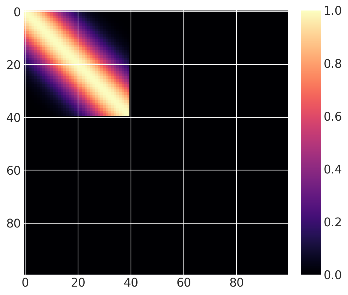
然后我们可以定义以下协方差函数，我们在\(x \in (0, 100)\)范围内计算它。 基础协方差的长度尺度为10，且\(x_0 = 40\)。 由于我们使用的是阶跃函数，当greater=False时，它在\(x \leq 40\)时“激活”，而当greater=True时，它在\(x > 40\)时“激活”。

cov = pm.gp.cov.ExpQuad(1, 10)
sc_cov = pm.gp.cov.ScaledCov(1, cov, step_function, (40, False))

x = np.linspace(0, 100, 100)
K = sc_cov(x[:, None]).eval()
m = plt.imshow(K, cmap="magma")
plt.colorbar(m);

/Users/alex_andorra/tptm_alex/pymc3/pymc3/gp/cov.py:93: UserWarning: Only 1 column(s) out of Subtensor{int64}.0 are being used to compute the covariance function. If this is not intended, increase 'input_dim' parameter to the number of columns to use. Ignore otherwise.
  " the number of columns to use. Ignore otherwise.", UserWarning)

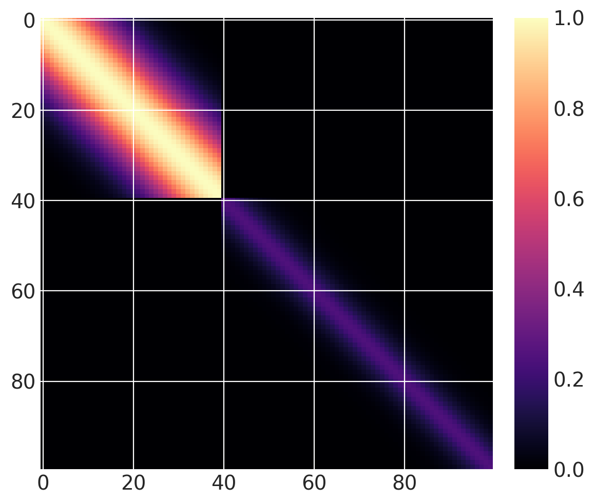
但这还不是变化点协方差函数。我们可以将两个这样的函数相加。对于 \(x > 40\)，让我们使用一个基协方差，它是具有长度尺度为 5 和幅度为 0.25 的 Matern32：

cov1 = pm.gp.cov.ExpQuad(1, 10)
sc_cov1 = pm.gp.cov.ScaledCov(1, cov1, step_function, (40, False))

cov2 = 0.25 * pm.gp.cov.Matern32(1, 5)
sc_cov2 = pm.gp.cov.ScaledCov(1, cov2, step_function, (40, True))

sc_cov = sc_cov1 + sc_cov2

# plot over 0 < x < 100
x = np.linspace(0, 100, 100)
K = sc_cov(x[:, None]).eval()
m = plt.imshow(K, cmap="magma")
plt.colorbar(m);

/Users/alex_andorra/tptm_alex/pymc3/pymc3/gp/cov.py:93: UserWarning: Only 1 column(s) out of Subtensor{int64}.0 are being used to compute the covariance function. If this is not intended, increase 'input_dim' parameter to the number of columns to use. Ignore otherwise.
  " the number of columns to use. Ignore otherwise.", UserWarning)
/Users/alex_andorra/tptm_alex/pymc3/pymc3/gp/cov.py:93: UserWarning: Only 1 column(s) out of Subtensor{int64}.0 are being used to compute the covariance function. If this is not intended, increase 'input_dim' parameter to the number of columns to use. Ignore otherwise.
  " the number of columns to use. Ignore otherwise.", UserWarning)

这个协方差的高斯过程先验样本是什么样子的？

prior_samples = np.random.multivariate_normal(np.zeros(100), K, 3).T
plt.plot(x, prior_samples)
plt.axvline(x=40, color="k", alpha=0.5);

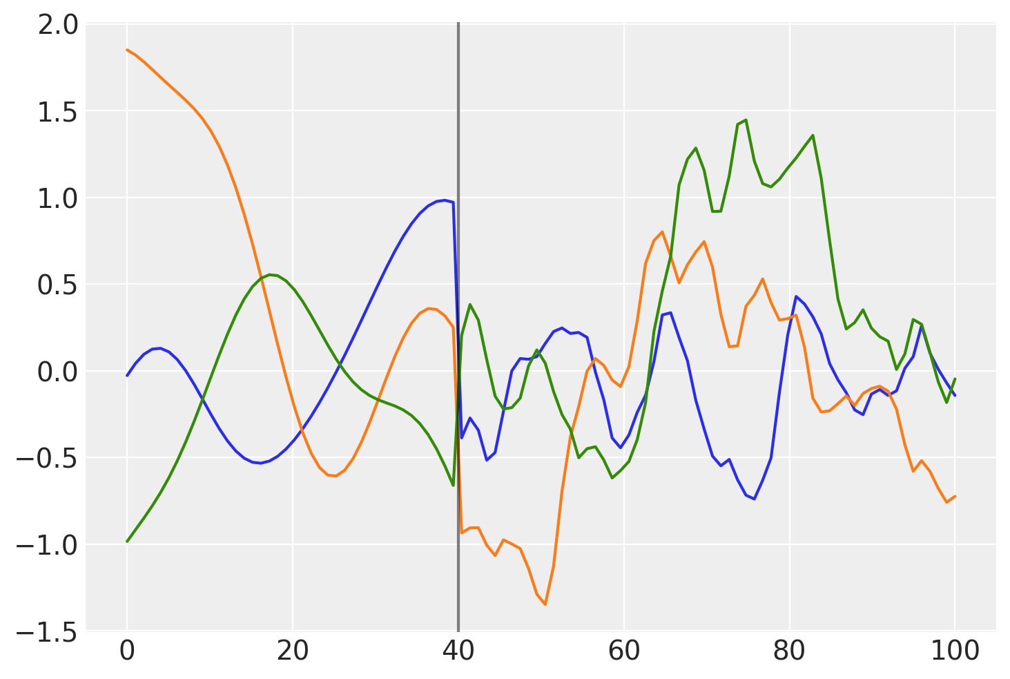
在 \(x = 40\) 之前，函数是平滑且缓慢变化的。在 \(x = 40\) 之后，样本变得不那么平滑且变化迅速。

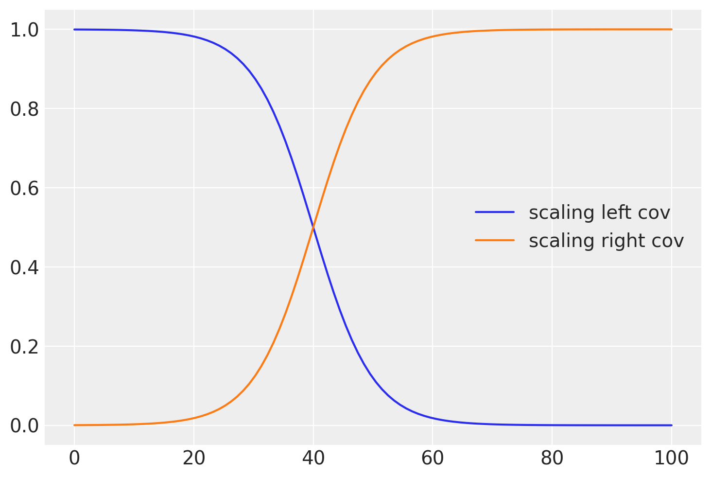
使用Sigmoid函数的渐进变化

与其使用一个明显的截止点，通常更现实的做法是有一个平滑的过渡。为此，我们可以使用逻辑函数，如下所示：

# b is the slope, a is the location

b = -0.2
a = 40
plt.plot(x, pm.math.invlogit(b * (x - a)).eval(), label="scaling left cov")

b = 0.2
a = 40
plt.plot(x, pm.math.invlogit(b * (x - a)).eval(), label="scaling right cov")
plt.legend();

def logistic(x, b, x0):
    # b is the slope, x0 is the location
    return pm.math.invlogit(b * (x - x0))

与之前相同的协方差函数，但带有一个逐渐变化点，如下所示：

cov1 = pm.gp.cov.ExpQuad(1, 10)
sc_cov1 = pm.gp.cov.ScaledCov(1, cov1, logistic, (-0.1, 40))

cov2 = 0.25 * pm.gp.cov.Matern32(1, 5)
sc_cov2 = pm.gp.cov.ScaledCov(1, cov2, logistic, (0.1, 40))

sc_cov = sc_cov1 + sc_cov2

# plot over 0 < x < 100
x = np.linspace(0, 100, 100)
K = sc_cov(x[:, None]).eval()
m = plt.imshow(K, cmap="magma")
plt.colorbar(m);

/Users/alex_andorra/tptm_alex/pymc3/pymc3/gp/cov.py:93: UserWarning: Only 1 column(s) out of Subtensor{int64}.0 are being used to compute the covariance function. If this is not intended, increase 'input_dim' parameter to the number of columns to use. Ignore otherwise.
  " the number of columns to use. Ignore otherwise.", UserWarning)

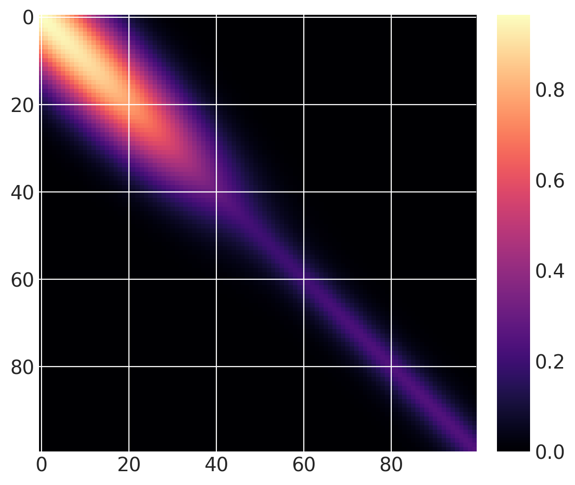
下面，你可以看到先验函数从一个区域到下一个区域的过渡更加渐进：

prior_samples = np.random.multivariate_normal(np.zeros(100), K, 3).T
plt.plot(x, prior_samples)
plt.axvline(x=40, color="k", alpha=0.5);

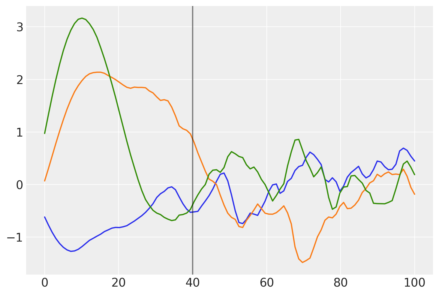
让我们尝试这个模型，而不是半参数变化点版本。

变化点协方差模型

该模型的特点是：

• 所有时间点短期变化的协方差

• 参数 x0 是工业革命发生的位置。它被赋予了一个先验分布，该分布的支持主要集中在1760年到1840年之间，中心在1800年。

• 我们可以轻松地将这个x0参数用作二阶多项式（二次）协方差中的平移参数，以及变化点协方差中的变化点位置。

• 工业革命前为ExpQuad的变点协方差，工业革命后为ExpQuad + Polynomial(degree=2)。

• 我们在变化点协方差中的两个基本协方差中使用相同的缩放和长度尺度参数。

• 仍然像之前一样对x中的不确定性进行建模。

with pm.Model() as model:
    η = pm.HalfNormal("η", sigma=5)
    ℓ = pm.Gamma("ℓ", alpha=2, beta=0.1)

    # changepoint occurs near the year 1800, sometime between 1760, 1840
    x0 = pm.Normal("x0", mu=18, sigma=0.1)
    # the change happens gradually
    a = pm.HalfNormal("a", sigma=2)
    # a constant for the
    c = pm.HalfNormal("c", sigma=3)
    # quadratic polynomial scale
    ηq = pm.HalfNormal("ηq", sigma=5)

    cov1 = η**2 * pm.gp.cov.ExpQuad(1, ℓ)
    cov2 = η**2 * pm.gp.cov.ExpQuad(1, ℓ) + ηq**2 * pm.gp.cov.Polynomial(1, x0, 2, c)

    # construct changepoint cov
    sc_cov1 = pm.gp.cov.ScaledCov(1, cov1, logistic, (-a, x0))
    sc_cov2 = pm.gp.cov.ScaledCov(1, cov2, logistic, (a, x0))
    cov_c = sc_cov1 + sc_cov2

    # short term variation
    ηs = pm.HalfNormal("ηs", sigma=5)
    ℓs = pm.Gamma("ℓs", alpha=2, beta=1)
    cov_s = ηs**2 * pm.gp.cov.Matern52(1, ℓs)

    gp = pm.gp.Marginal(cov_func=cov_s + cov_c)

    t_diff = pm.Normal("t_diff", mu=0.0, sigma=0.02, shape=len(t))
    t_uncert = t_n - t_diff

    # white noise variance
    σ = pm.HalfNormal("σ", sigma=5, testval=1)
    y_ = gp.marginal_likelihood("y", X=t_uncert[:, None], y=y_n, noise=σ)

/Users/alex_andorra/tptm_alex/pymc3/pymc3/gp/cov.py:93: UserWarning: Only 1 column(s) out of Subtensor{int64}.0 are being used to compute the covariance function. If this is not intended, increase 'input_dim' parameter to the number of columns to use. Ignore otherwise.
  " the number of columns to use. Ignore otherwise.", UserWarning)
/Users/alex_andorra/tptm_alex/pymc3/pymc3/gp/cov.py:93: UserWarning: Only 1 column(s) out of Subtensor{int64}.0 are being used to compute the covariance function. If this is not intended, increase 'input_dim' parameter to the number of columns to use. Ignore otherwise.
  " the number of columns to use. Ignore otherwise.", UserWarning)
/Users/alex_andorra/tptm_alex/pymc3/pymc3/gp/cov.py:93: UserWarning: Only 1 column(s) out of Subtensor{int64}.0 are being used to compute the covariance function. If this is not intended, increase 'input_dim' parameter to the number of columns to use. Ignore otherwise.
  " the number of columns to use. Ignore otherwise.", UserWarning)

with model:
    tr = pm.sample(500, chains=2, target_accept=0.95)

Auto-assigning NUTS sampler...
Initializing NUTS using jitter+adapt_diag...
Multiprocess sampling (2 chains in 4 jobs)
NUTS: [σ, t_diff, ℓs, ηs, ηq, c, a, x0, ℓ, η]

100.00% [3000/3000 02:27<00:00 Sampling 2 chains, 0 divergences]

Sampling 2 chains for 1_000 tune and 500 draw iterations (2_000 + 1_000 draws total) took 151 seconds.

az.plot_trace(tr, var_names=["η", "ηs", "ℓ", "ℓs", "c", "a", "x0", "σ"]);

/Users/alex_andorra/opt/anaconda3/envs/dev-pymc/lib/python3.6/site-packages/arviz/data/io_pymc3.py:89: FutureWarning: Using `from_pymc3` without the model will be deprecated in a future release. Not using the model will return less accurate and less useful results. Make sure you use the model argument or call from_pymc3 within a model context.
  FutureWarning,

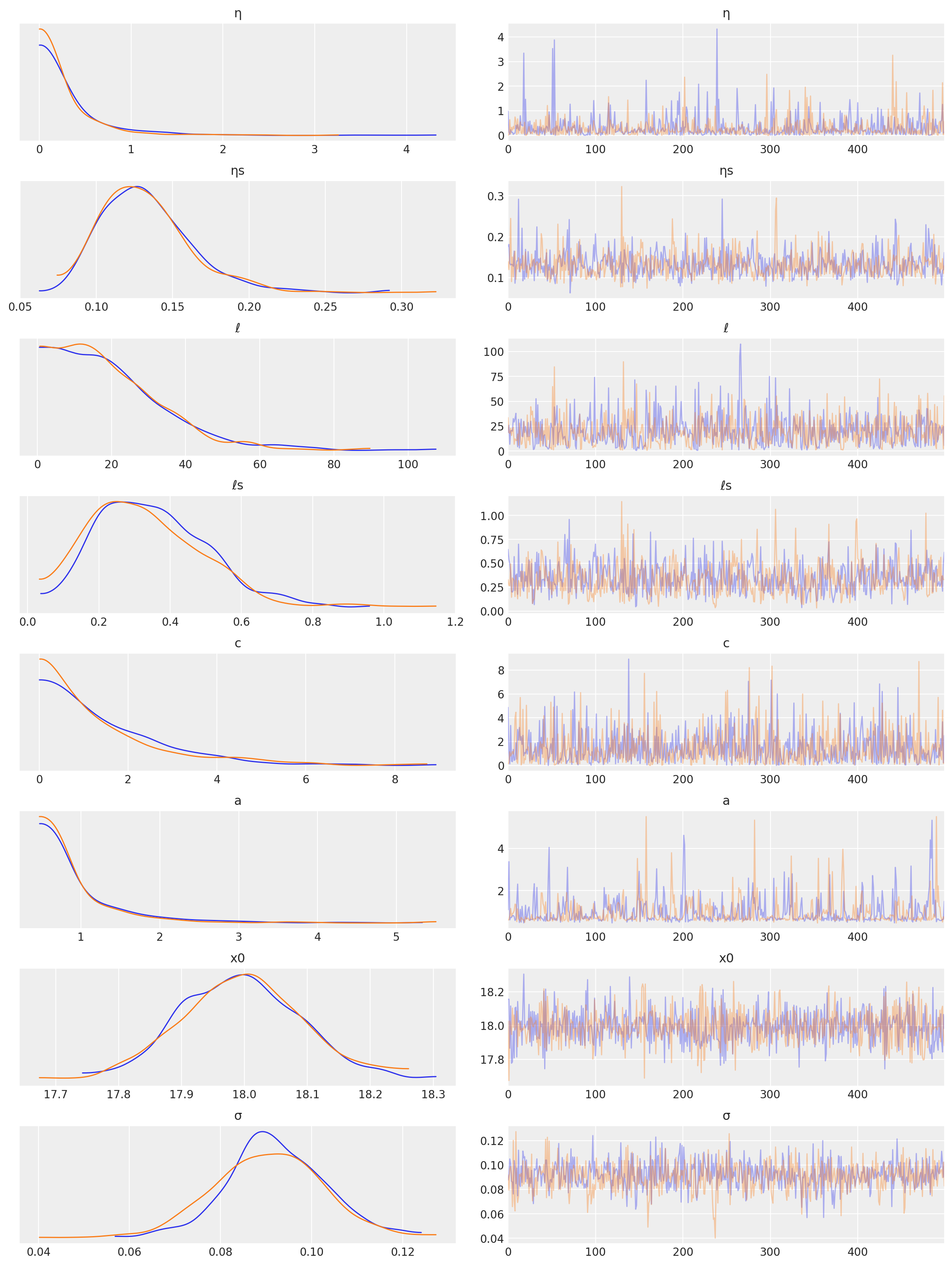
预测

tnew = np.linspace(-100, 2300, 2200) * 0.01

with model:
    fnew = gp.conditional("fnew", Xnew=tnew[:, None])

with model:
    ppc = pm.sample_posterior_predictive(tr, samples=100, var_names=["fnew"])

/Users/alex_andorra/tptm_alex/pymc3/pymc3/gp/cov.py:93: UserWarning: Only 1 column(s) out of Subtensor{int64}.0 are being used to compute the covariance function. If this is not intended, increase 'input_dim' parameter to the number of columns to use. Ignore otherwise.
  " the number of columns to use. Ignore otherwise.", UserWarning)
/Users/alex_andorra/tptm_alex/pymc3/pymc3/sampling.py:1708: UserWarning: samples parameter is smaller than nchains times ndraws, some draws and/or chains may not be represented in the returned posterior predictive sample
  "samples parameter is smaller than nchains times ndraws, some draws "

100.00% [100/100 06:35<00:00]

samples = y_sd * ppc["fnew"] + y_mu

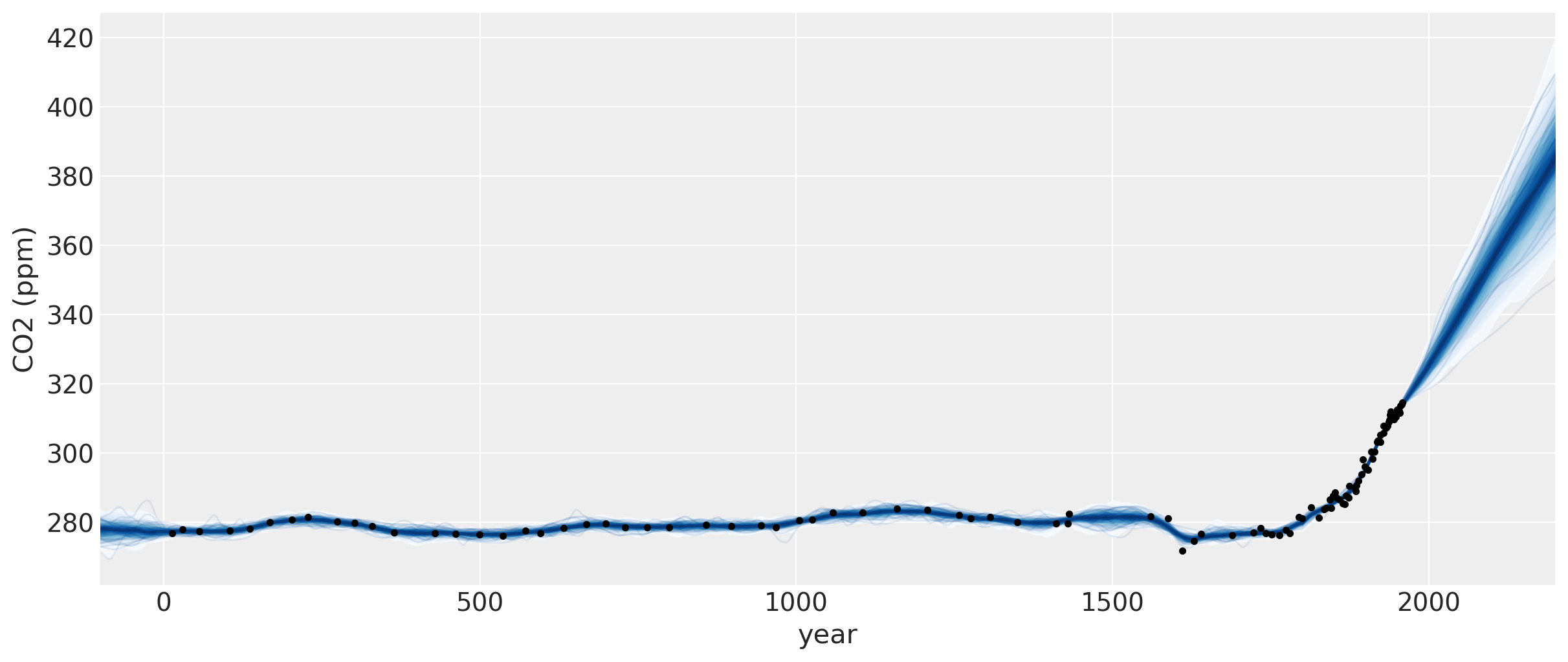
fig = plt.figure(figsize=(12, 5))
ax = plt.gca()
pm.gp.util.plot_gp_dist(ax, samples, tnew, plot_samples=True, palette="Blues")
ax.plot(t / 100, y, "k.")
ax.set_xticks(np.arange(0, 23))
ax.set_xlim([-1, 23])
ax.set_ylim([250, 450])
ax.set_xlabel("time (in centuries)")
ax.set_ylabel("CO2 (ppm)");

该模型的预测看起来更加真实。一个二次多项式与ExpQuad的和看起来是一个很好的预测模型。它允许二氧化碳的量以非完全线性的方式增加。从预测中我们可以看出：

• 二氧化碳的量可能会以更快的速度增加

• 二氧化碳的量应该或多或少地线性增加

• 二氧化碳有可能开始减少

结合大气CO2测量数据

接下来，我们将结合来自Mauna Loa观测站的CO2测量数据。这些数据点是从大气层中每月采集的。与冰芯数据不同，这些测量数据没有不确定性。在同时建模这两组数据时，包含冰芯测量时间的不确定性将变得更加明显。使用冰芯数据来预测Mauna Loa的季节性变化并没有太大意义，因为南极的季节性模式与夏威夷北半球的模式不同。不过，我们还是会展示它，因为这是可能的，并且在其他情况下可能会有用。

首先让我们加载数据，然后将其与冰芯数据一起绘制。

import time

from datetime import datetime as dt


def toYearFraction(date):
    date = pd.to_datetime(date)

    def sinceEpoch(date):  # returns seconds since epoch
        return time.mktime(date.timetuple())

    s = sinceEpoch

    year = date.year
    startOfThisYear = dt(year=year, month=1, day=1)
    startOfNextYear = dt(year=year + 1, month=1, day=1)

    yearElapsed = s(date) - s(startOfThisYear)
    yearDuration = s(startOfNextYear) - s(startOfThisYear)
    fraction = yearElapsed / yearDuration

    return date.year + fraction

airdata = pd.read_csv(pm.get_data("monthly_in_situ_co2_mlo.csv"), header=56)

# - replace -99.99 with NaN
airdata.replace(to_replace=-99.99, value=np.nan, inplace=True)

# fix column names
cols = [
    "year",
    "month",
    "--",
    "--",
    "CO2",
    "seasonaly_adjusted",
    "fit",
    "seasonally_adjusted_fit",
    "CO2_filled",
    "seasonally_adjusted_filled",
]
airdata.columns = cols
cols.remove("--")
cols.remove("--")
airdata = airdata[cols]

# drop rows with nan
airdata.dropna(inplace=True)

# fix time index
airdata["day"] = 15
airdata.index = pd.to_datetime(airdata[["year", "month", "day"]])
airdata["year"] = [toYearFraction(date) for date in airdata.index.values]
cols.remove("month")
airdata = airdata[cols]

air = airdata[["year", "CO2"]]
air.head(5)

	year	CO2
1958-03-15	1958.200000	315.69
1958-04-15	1958.284932	317.46
1958-05-15	1958.367123	317.50
1958-07-15	1958.534247	315.86
1958-08-15	1958.619178	314.93

与在第一个笔记本中完成的一样，我们将2004年以后的数据保留为测试集。

sep_idx = air.index.searchsorted(pd.to_datetime("2003-12-15"))
air_test = air.iloc[sep_idx:, :]
air = air.iloc[: sep_idx + 1, :]

plt.plot(air.year.values, air.CO2.values, ".b", label="atmospheric CO2")
plt.plot(ice.year.values, ice.CO2.values, ".", color="c", label="ice core CO2")
plt.legend()
plt.xlabel("year")
plt.ylabel("CO2 (ppm)");

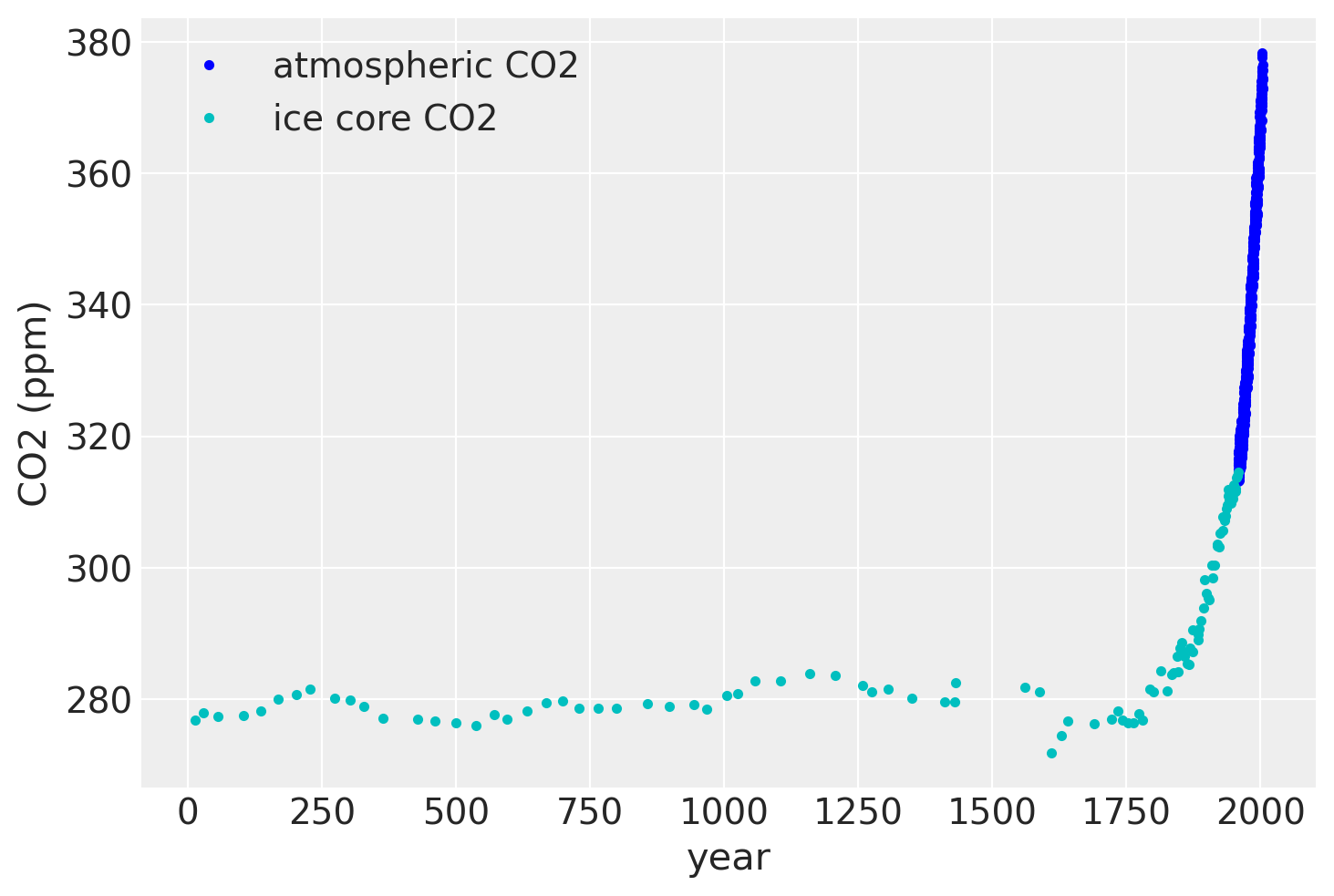
如果我们放大到20世纪50年代末，我们可以看到大气数据具有季节性成分，而冰芯数据则没有。

plt.plot(air.year.values, air.CO2.values, ".b", label="atmospheric CO2")
plt.plot(ice.year.values, ice.CO2.values, ".", color="c", label="ice core CO2")
plt.xlim([1949, 1965])
plt.ylim([305, 325])
plt.legend()
plt.xlabel("year")
plt.ylabel("CO2 (ppm)");

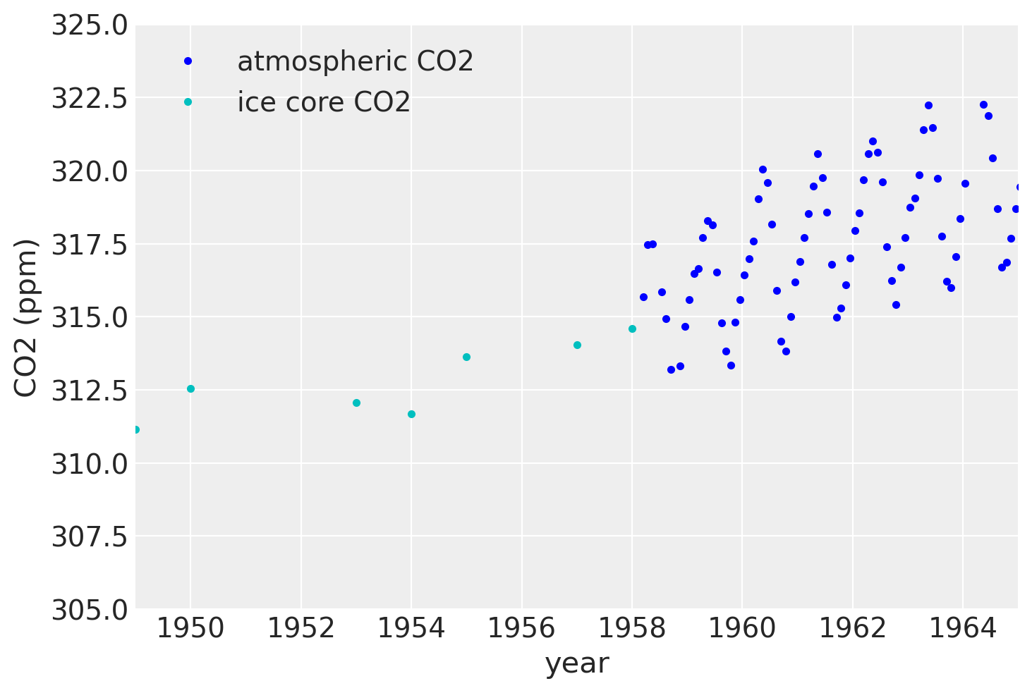
由于冰芯数据测量不准确，除非我们建模不确定性在x中，否则无法回溯季节性成分。

为了同时对数据进行建模，我们将结合使用冰芯数据构建的模型，并将其与前一个关于莫纳罗亚数据的笔记本中的元素结合起来。从前一个笔记本中，我们还将包括：

• 周期性，季节性成分

• 用于短程、年度尺度变化的 RatQuad 协方差

此外，由于我们使用了两个不同的数据集，因此应该有两个不同的y方向的不确定性，一个是针对冰芯数据的，另一个是针对大气数据的。为了实现这一点，我们创建了一个自定义的WhiteNoise协方差函数，该函数具有两个σ参数。

所有自定义协方差函数都需要定义相同的三种方法，__init__、diag 和 full。full 返回完整的协方差，给定 X 或 X 和不同的 Xs。diag 仅返回对角线，而 __init__ 保存输入参数。

class CustomWhiteNoise(pm.gp.cov.Covariance):
    """Custom White Noise covariance
    - sigma1 is applied to the first n1 points in the data
    - sigma2 is applied to the next n2 points in the data

    The total number of data points n = n1 + n2
    """

    def __init__(self, sigma1, sigma2, n1, n2):
        super().__init__(1, None)
        self.sigma1 = sigma1
        self.sigma2 = sigma2
        self.n1 = n1
        self.n2 = n2

    def diag(self, X):
        d1 = tt.alloc(tt.square(self.sigma1), self.n1)
        d2 = tt.alloc(tt.square(self.sigma2), self.n2)
        return tt.concatenate((d1, d2), 0)

    def full(self, X, Xs=None):
        if Xs is None:
            return tt.diag(self.diag(X))
        else:
            return tt.alloc(0.0, X.shape[0], Xs.shape[0])

接下来我们需要组织并合并这两个数据集。请记住，x轴的单位是世纪，而不是年份。

# form dataset, stack t and co2 measurements
t = np.concatenate((ice.year.values, air.year.values), 0)
y = np.concatenate((ice.CO2.values, air.CO2.values), 0)

y_mu, y_sd = np.mean(ice.CO2.values[0:50]), np.std(y)
y_n = (y - y_mu) / y_sd
t_n = t * 0.01

模型的规格如下。现在数据集更大了，所以MCMC会花费更长的时间。但你将会看到，估计整个后验分布显然是值得等待的！

我们也更仔细地选择了超参数的先验。对于变化点的协方差，我们使用与工业革命前相同的长尺度ExpQuad协方差来建模工业革命后的数据。这个想法是，无论工业革命前是什么过程在起作用，工业革命后仍然存在。但随后我们添加了Polynomial(degree=2)和Matern52的乘积。我们将Matern52的长度尺度固定为2。由于工业革命至今只有大约两个世纪，我们强制多项式成分在这个时间尺度上衰减。这迫使不确定性在这个时间尺度上上升。

二阶多项式和 Matern52 乘积表达了我们先验的信念，即二氧化碳水平可能会半二次方增加，或半二次方减少，因为该比例参数最终也可能为零。

with pm.Model() as model:
    ηc = pm.Gamma("ηc", alpha=3, beta=2)
    ℓc = pm.Gamma("ℓc", alpha=10, beta=1)

    # changepoint occurs near the year 1800, sometime between 1760, 1840
    x0 = pm.Normal("x0", mu=18, sigma=0.1)
    # the change happens gradually
    a = pm.Gamma("a", alpha=3, beta=1)
    # constant offset
    c = pm.HalfNormal("c", sigma=2)

    # quadratic polynomial scale
    ηq = pm.HalfNormal("ηq", sigma=1)
    ℓq = 2.0  # 2 century impact, since we only have 2 C of post IR data

    cov1 = ηc**2 * pm.gp.cov.ExpQuad(1, ℓc)
    cov2 = ηc**2 * pm.gp.cov.ExpQuad(1, ℓc) + ηq**2 * pm.gp.cov.Polynomial(
        1, x0, 2, c
    ) * pm.gp.cov.Matern52(
        1, ℓq
    )  # ~2 century impact

    # construct changepoint cov
    sc_cov1 = pm.gp.cov.ScaledCov(1, cov1, logistic, (-a, x0))
    sc_cov2 = pm.gp.cov.ScaledCov(1, cov2, logistic, (a, x0))
    gp_c = pm.gp.Marginal(cov_func=sc_cov1 + sc_cov2)

    # short term variation
    ηs = pm.HalfNormal("ηs", sigma=3)
    ℓs = pm.Gamma("ℓs", alpha=5, beta=100)
    α = pm.Gamma("α", alpha=4, beta=1)
    cov_s = ηs**2 * pm.gp.cov.RatQuad(1, α, ℓs)
    gp_s = pm.gp.Marginal(cov_func=cov_s)

    # medium term variation
    ηm = pm.HalfNormal("ηm", sigma=5)
    ℓm = pm.Gamma("ℓm", alpha=2, beta=3)
    cov_m = ηm**2 * pm.gp.cov.ExpQuad(1, ℓm)
    gp_m = pm.gp.Marginal(cov_func=cov_m)

    ## periodic
    ηp = pm.HalfNormal("ηp", sigma=2)
    ℓp_decay = pm.Gamma("ℓp_decay", alpha=40, beta=0.1)
    ℓp_smooth = pm.Normal("ℓp_smooth ", mu=1.0, sigma=0.05)
    period = 1 * 0.01  # we know the period is annual
    cov_p = ηp**2 * pm.gp.cov.Periodic(1, period, ℓp_smooth) * pm.gp.cov.ExpQuad(1, ℓp_decay)
    gp_p = pm.gp.Marginal(cov_func=cov_p)

    gp = gp_c + gp_m + gp_s + gp_p

    # - x location uncertainty (sd = 0.01 is a standard deviation of one year)
    # - only the first 111 points are the ice core data
    t_mu = t_n[:111]
    t_diff = pm.Normal("t_diff", mu=0.0, sigma=0.02, shape=len(t_mu))
    t_uncert = t_mu - t_diff
    t_combined = tt.concatenate((t_uncert, t_n[111:]), 0)

    # Noise covariance, using boundary avoiding priors for MAP estimation
    σ1 = pm.Gamma("σ1", alpha=3, beta=50)
    σ2 = pm.Gamma("σ2", alpha=3, beta=50)
    η_noise = pm.HalfNormal("η_noise", sigma=1)
    ℓ_noise = pm.Gamma("ℓ_noise", alpha=2, beta=200)
    cov_noise = η_noise**2 * pm.gp.cov.Matern32(1, ℓ_noise) + CustomWhiteNoise(σ1, σ2, 111, 545)

    y_ = gp.marginal_likelihood("y", X=t_combined[:, None], y=y_n, noise=cov_noise)

/Users/alex_andorra/tptm_alex/pymc3/pymc3/gp/cov.py:93: UserWarning: Only 1 column(s) out of Subtensor{int64}.0 are being used to compute the covariance function. If this is not intended, increase 'input_dim' parameter to the number of columns to use. Ignore otherwise.
  " the number of columns to use. Ignore otherwise.", UserWarning)
/Users/alex_andorra/tptm_alex/pymc3/pymc3/gp/cov.py:93: UserWarning: Only 1 column(s) out of Subtensor{int64}.0 are being used to compute the covariance function. If this is not intended, increase 'input_dim' parameter to the number of columns to use. Ignore otherwise.
  " the number of columns to use. Ignore otherwise.", UserWarning)
/Users/alex_andorra/tptm_alex/pymc3/pymc3/gp/cov.py:93: UserWarning: Only 1 column(s) out of Subtensor{int64}.0 are being used to compute the covariance function. If this is not intended, increase 'input_dim' parameter to the number of columns to use. Ignore otherwise.
  " the number of columns to use. Ignore otherwise.", UserWarning)

with model:
    tr = pm.sample(500, tune=1000, chains=2, cores=16, return_inferencedata=True)

Auto-assigning NUTS sampler...
Initializing NUTS using jitter+adapt_diag...
Multiprocess sampling (2 chains in 16 jobs)
NUTS: [ℓ_noise, η_noise, σ2, σ1, t_diff, ℓp_smooth , ℓp_decay, ηp, ℓm, ηm, α, ℓs, ηs, ηq, c, a, x0, ℓc, ηc]

100.00% [3000/3000 21:58:11<00:00 Sampling 2 chains, 17 divergences]

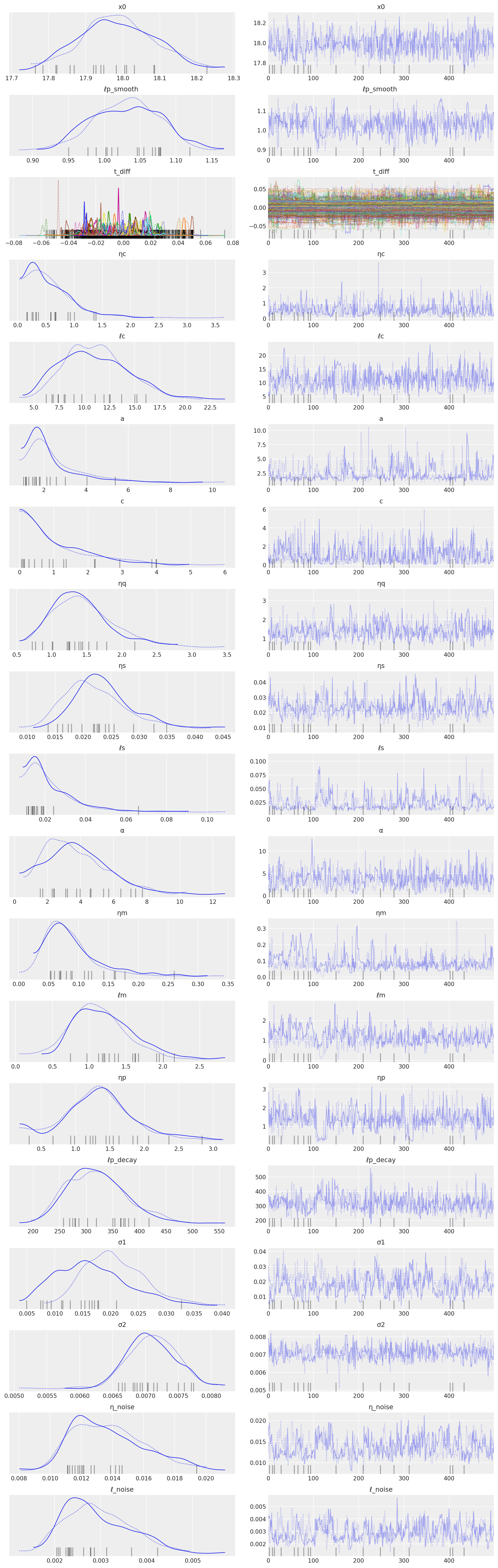
Sampling 2 chains for 1_000 tune and 500 draw iterations (2_000 + 1_000 draws total) took 79100 seconds.
There were 17 divergences after tuning. Increase `target_accept` or reparameterize.
The rhat statistic is larger than 1.4 for some parameters. The sampler did not converge.
The estimated number of effective samples is smaller than 200 for some parameters.

az.plot_trace(tr, compact=True);

/Users/alex_andorra/opt/anaconda3/envs/dev-pymc/lib/python3.6/site-packages/arviz/data/io_pymc3.py:89: FutureWarning: Using `from_pymc3` without the model will be deprecated in a future release. Not using the model will return less accurate and less useful results. Make sure you use the model argument or call from_pymc3 within a model context.
  FutureWarning,

tnew = np.linspace(1700, 2040, 3000) * 0.01
with model:
    fnew = gp.conditional("fnew", Xnew=tnew[:, None])

/Users/alex_andorra/tptm_alex/pymc3/pymc3/gp/cov.py:93: UserWarning: Only 1 column(s) out of Subtensor{int64}.0 are being used to compute the covariance function. If this is not intended, increase 'input_dim' parameter to the number of columns to use. Ignore otherwise.
  " the number of columns to use. Ignore otherwise.", UserWarning)

with model:
    ppc = pm.sample_posterior_predictive(tr, samples=200, var_names=["fnew"])

/Users/alex_andorra/tptm_alex/pymc3/pymc3/sampling.py:1708: UserWarning: samples parameter is smaller than nchains times ndraws, some draws and/or chains may not be represented in the returned posterior predictive sample
  "samples parameter is smaller than nchains times ndraws, some draws "

100.00% [200/200 46:10<00:00]

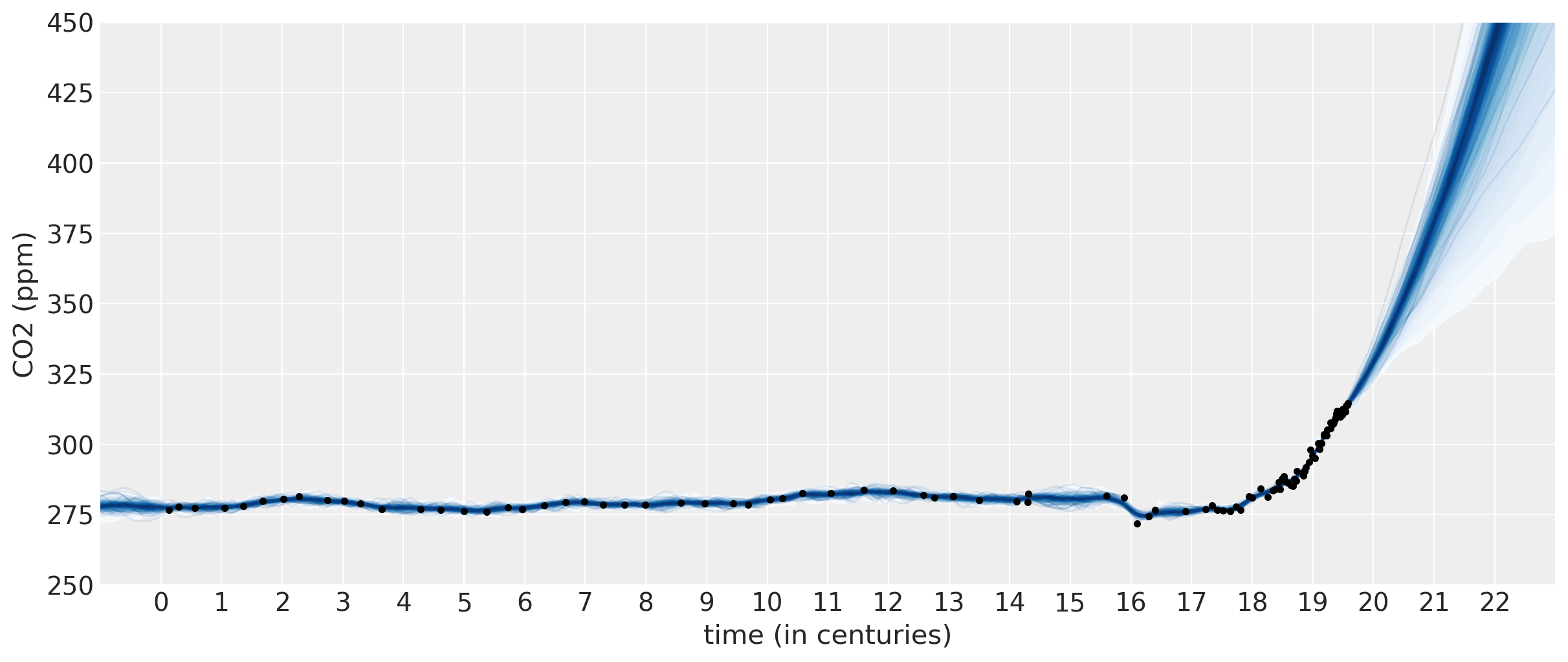
以下是自18世纪以来用于拟合模型的数据图（Mauna Loa和Law Dome冰芯数据）。浅蓝色线条在这个缩放级别下有点难以辨认，但它们是高斯过程后验的样本。它们既插值了观测数据，也代表了未来预测的合理轨迹。这些样本也可以用来定义置信区间。

plt.figure(figsize=(12, 5))
plt.plot(tnew * 100, y_sd * ppc["fnew"][0:200:5, :].T + y_mu, color="lightblue", alpha=0.8)
plt.plot(
    [-1000, -1001],
    [-1000, -1001],
    color="lightblue",
    alpha=0.8,
    label="samples from the posterior",
)
plt.plot(t, y, "k.", label="observed data")
plt.plot(
    air_test.year.values,
    air_test.CO2.values,
    ".",
    color="orange",
    label="test set data",
)
plt.axhline(y=400, color="k", alpha=0.7, linestyle=":")
plt.ylabel("CO2 [ppm]")
plt.xlabel("year")
plt.title("fit and possible forecasts")
plt.legend()
plt.xlim([1700, 2040])
plt.ylim([260, 460]);

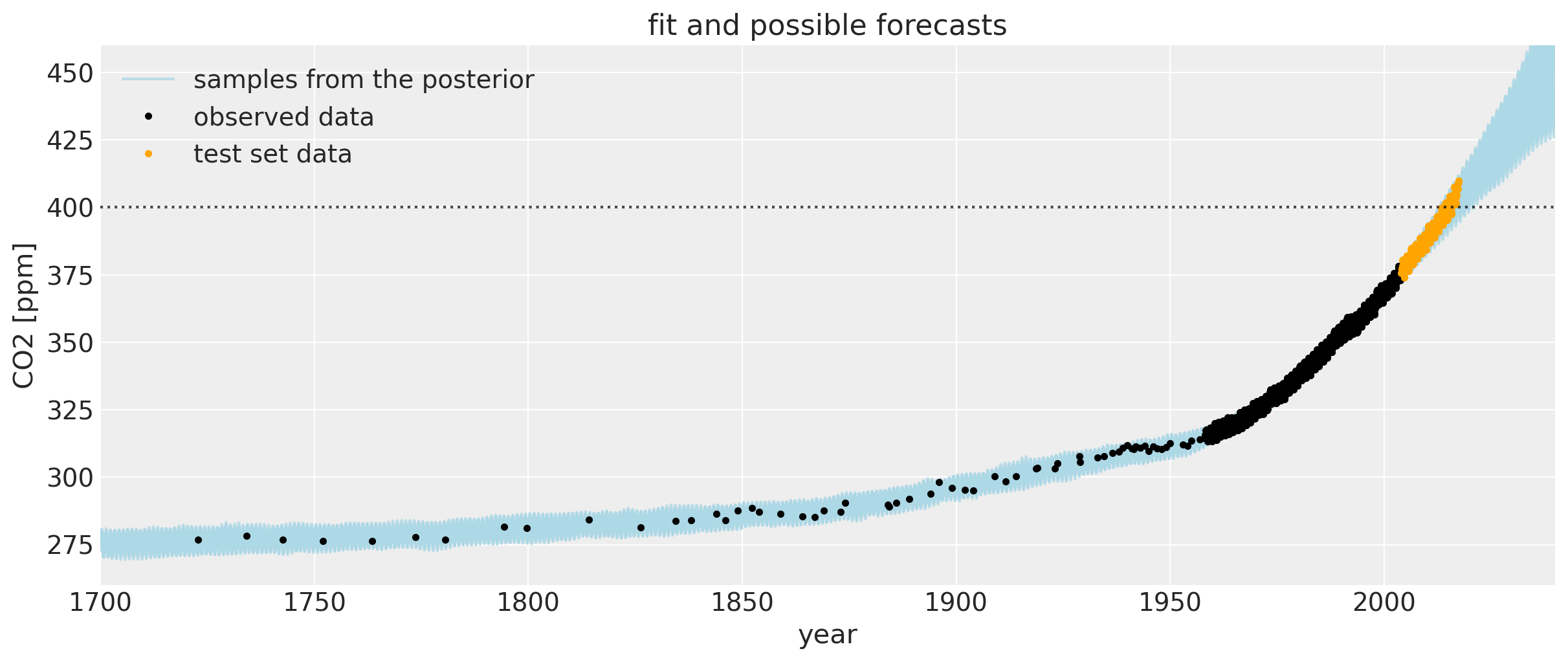
让我们放大一下，更仔细地观察CO2水平首次超过400 ppm时周围区域的不确定区间。我们可以看到后验样本给出了一个合理的未来轨迹范围。请注意，图中橙色绘制的数据并未用于模型拟合。

plt.figure(figsize=(12, 5))
plt.plot(tnew * 100, y_sd * ppc["fnew"][0:200:5, :].T + y_mu, color="lightblue", alpha=0.8)
plt.plot(
    [-1000, -1001],
    [-1000, -1001],
    color="lightblue",
    alpha=0.8,
    label="samples from the posterior",
)
plt.plot(
    air_test.year.values,
    air_test.CO2.values,
    ".",
    color="orange",
    label="test set data",
)
plt.axhline(y=400, color="k", alpha=0.7, linestyle=":")
plt.ylabel("CO2 [ppm]")
plt.xlabel("year")
plt.title("fit and possible forecasts")
plt.legend()
plt.xlim([2004, 2040])
plt.ylim([360, 460]);

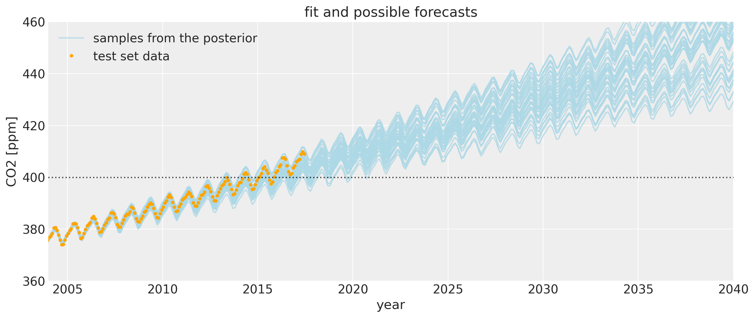
如果你将这个与第一个Mauna Loa示例笔记本进行比较，预测结果要好得多。预测CO2水平首次达到400的日期要准确得多。这种偏差的改进是由于包含了多项式 * Matern52项和变化点模型。

我们也可以看看模型对过去二氧化碳水平的描述。由于我们允许x测量值具有不确定性，因此我们能够将季节性成分拟合到过去。可以肯定的是，从科学的角度来看，使用冰芯数据对莫纳罗亚二氧化碳测量值进行回溯预测并没有太大意义，因为由于季节性变化，二氧化碳水平会因您在地球上的位置而异。莫纳罗亚的周期性模式会更加明显，因为北半球拥有更多的植被。植被的多少在很大程度上驱动了季节性变化，这是由于植物在夏季和冬季的生长和凋零。但正因为这很酷，我们还是来看看这里的模型拟合情况吧：

tnew = np.linspace(11, 32, 500) * 0.01
with model:
    fnew2 = gp.conditional("fnew2", Xnew=tnew[:, None])

/Users/alex_andorra/tptm_alex/pymc3/pymc3/gp/cov.py:93: UserWarning: Only 1 column(s) out of Subtensor{int64}.0 are being used to compute the covariance function. If this is not intended, increase 'input_dim' parameter to the number of columns to use. Ignore otherwise.
  " the number of columns to use. Ignore otherwise.", UserWarning)

with model:
    ppc = pm.sample_posterior_predictive(tr, samples=200, var_names=["fnew2"])

/Users/alex_andorra/tptm_alex/pymc3/pymc3/sampling.py:1708: UserWarning: samples parameter is smaller than nchains times ndraws, some draws and/or chains may not be represented in the returned posterior predictive sample
  "samples parameter is smaller than nchains times ndraws, some draws "

100.00% [200/200 01:08<00:00]

plt.figure(figsize=(12, 5))

plt.plot(tnew * 100, y_sd * ppc["fnew2"][0:200:10, :].T + y_mu, color="lightblue", alpha=0.8)
plt.plot(
    [-1000, -1001],
    [-1000, -1001],
    color="lightblue",
    alpha=0.8,
    label="samples from the GP posterior",
)
plt.plot(100 * (t_n[:111][:, None] - tr["t_diff"].T), y[:111], "oy", alpha=0.01)
plt.plot(
    [100, 200],
    [100, 200],
    "oy",
    alpha=0.3,
    label="data location posterior samples reflecting ice core time measurement uncertainty",
)
plt.plot(t, y, "k.", label="observed data")
plt.plot(air_test.year.values, air_test.CO2.values, ".", color="orange")
plt.legend(loc="upper left")
plt.ylabel("CO2 [ppm]")
plt.xlabel("year")
plt.xlim([12, 31])
plt.xticks(np.arange(12, 32))
plt.ylim([272, 283]);

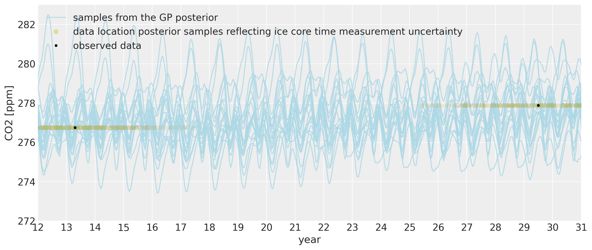
我们可以看到，即使在遥远的过去，我们也可以在一定程度上回溯季节性行为。在x位置的约两年不确定性允许它们被移动到该年季节性振荡的最近部分。振荡的幅度与现代时期相同。虽然每个后验样本中的周期仍然是年度周期，但由于我们距离收集莫纳罗亚数据的时间很远，其确切的形态不太确定。

tnew = np.linspace(-20, 0, 300) * 0.01
with model:
    fnew3 = gp.conditional("fnew3", Xnew=tnew[:, None])

/Users/alex_andorra/tptm_alex/pymc3/pymc3/gp/cov.py:93: UserWarning: Only 1 column(s) out of Subtensor{int64}.0 are being used to compute the covariance function. If this is not intended, increase 'input_dim' parameter to the number of columns to use. Ignore otherwise.
  " the number of columns to use. Ignore otherwise.", UserWarning)

with model:
    ppc = pm.sample_posterior_predictive(tr, samples=200, var_names=["fnew3"])

/Users/alex_andorra/tptm_alex/pymc3/pymc3/sampling.py:1708: UserWarning: samples parameter is smaller than nchains times ndraws, some draws and/or chains may not be represented in the returned posterior predictive sample
  "samples parameter is smaller than nchains times ndraws, some draws "

100.00% [200/200 00:52<00:00]

plt.figure(figsize=(12, 5))

plt.plot(tnew * 100, y_sd * ppc["fnew3"][0:200:10, :].T + y_mu, color="lightblue", alpha=0.8)
plt.plot(
    [-1000, -1001],
    [-1000, -1001],
    color="lightblue",
    alpha=0.8,
    label="samples from the GP posterior",
)
plt.legend(loc="upper left")
plt.ylabel("CO2 [ppm]")
plt.xlabel("year")
plt.xlim([-20, 0])
plt.ylim([272, 283]);

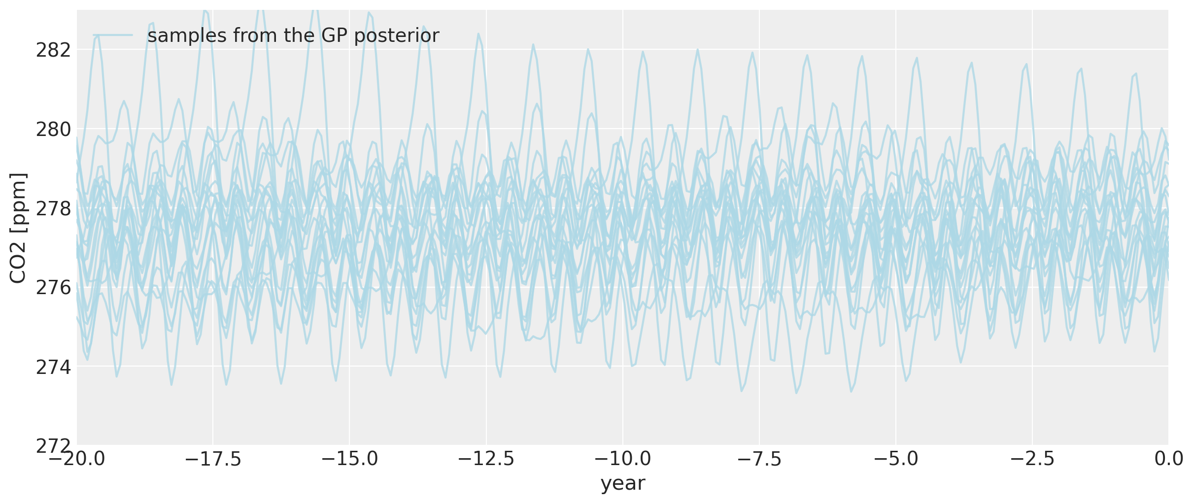
即使我们追溯到公元前零年之前，总体的回溯季节性模式仍然保持不变，尽管它开始变得更加剧烈地变化。

结论

本笔记本的目标是帮助提供一些利用 PyMC3 的 GP 建模能力的灵活性的方法。数据很少以整齐、均匀采样的间隔从一个单一来源中获取，但这对于 GP 模型来说通常不是问题。为了实现建模有趣行为，定义自定义协方差和均值函数非常容易。无需担心计算梯度，因为这是由 Theano 的自动微分功能处理的。能够在 PyMC3 中使用高质量的 NUTS 采样器进行 GP 模型意味着可以使用后验分布的样本作为可能的预测，这些预测考虑了均值和协方差函数超参数的不确定性。

%load_ext watermark
%watermark -n -u -v -iv -w

theano 1.0.5
pandas 1.1.0
numpy  1.19.1
pymc3  3.9.3
arviz  0.9.0
last updated: Sun Aug 09 2020 

CPython 3.6.11
IPython 7.16.1
watermark 2.0.2