稀疏近似

gp.MarginalSparse 类实现了稀疏或引导点的高斯过程近似。它的工作方式与 gp.Marginal 相同，只是它还需要引导点的位置（表示为 Xu），并且它接受参数 sigma 而不是 noise，因为这些稀疏近似假设白噪声是独立同分布的。

目前实现了三种近似方法：FITC、DTC 和 VFE。对于大多数问题，它们产生的结果相当相似。这些 GP 近似方法不会形成所有 \(n\) 个训练输入的完整协方差矩阵。相反，它们依赖于 \(m < n\) 个诱导点，这些点在整个域中“战略性”地分布。这两种近似方法都将 GP 的 \(\mathcal{O(n^3)}\) 复杂度降低到 \(\mathcal{O(nm^2)}\) —— 这是一个显著的速度提升。内存需求也有所减少，但减少的幅度不大。它们通常被称为稀疏近似，从数据稀疏的意义上来说。稀疏近似的缺点是它们降低了 GP 的表达能力。减少协方差矩阵的维度实际上减少了可以用来拟合数据的协方差矩阵特征向量的数量。

需要做出的选择是诱导点的放置位置。一种选择是使用输入的子集。另一种可能性是使用K均值。诱导点的位置也可以是未知的，并作为模型的一部分进行优化。这些稀疏近似在数据点密度高且长度尺度大于诱导点之间分离时，有助于加快计算速度。

有关这些近似的更多信息，请参阅 Quinonero-Candela+Rasmussen, 2006 和 Titsias 2009。

示例

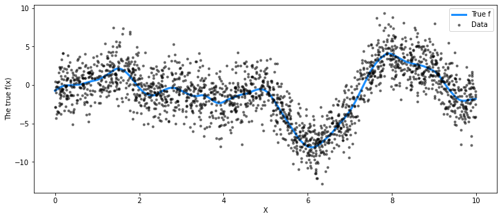
对于以下示例，我们使用与gp.Marginal示例中相同的数据集，但数据点更多。

import matplotlib.pyplot as plt
import numpy as np
import pymc3 as pm
import theano
import theano.tensor as tt

%matplotlib inline

# set the seed
np.random.seed(1)

n = 2000  # The number of data points
X = 10 * np.sort(np.random.rand(n))[:, None]

# Define the true covariance function and its parameters
ℓ_true = 1.0
η_true = 3.0
cov_func = η_true**2 * pm.gp.cov.Matern52(1, ℓ_true)

# A mean function that is zero everywhere
mean_func = pm.gp.mean.Zero()

# The latent function values are one sample from a multivariate normal
# Note that we have to call `eval()` because PyMC3 built on top of Theano
f_true = np.random.multivariate_normal(
    mean_func(X).eval(), cov_func(X).eval() + 1e-8 * np.eye(n), 1
).flatten()

# The observed data is the latent function plus a small amount of IID Gaussian noise
# The standard deviation of the noise is `sigma`
σ_true = 2.0
y = f_true + σ_true * np.random.randn(n)

## Plot the data and the unobserved latent function
fig = plt.figure(figsize=(12, 5))
ax = fig.gca()
ax.plot(X, f_true, "dodgerblue", lw=3, label="True f")
ax.plot(X, y, "ok", ms=3, alpha=0.5, label="Data")
ax.set_xlabel("X")
ax.set_ylabel("The true f(x)")
plt.legend();

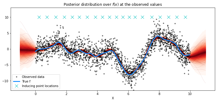
使用K-means初始化诱导点

我们使用NUTS采样器和FITC近似。

with pm.Model() as model:
    ℓ = pm.Gamma("ℓ", alpha=2, beta=1)
    η = pm.HalfCauchy("η", beta=5)

    cov = η**2 * pm.gp.cov.Matern52(1, ℓ)
    gp = pm.gp.MarginalSparse(cov_func=cov, approx="FITC")

    # initialize 20 inducing points with K-means
    # gp.util
    Xu = pm.gp.util.kmeans_inducing_points(20, X)

    σ = pm.HalfCauchy("σ", beta=5)
    y_ = gp.marginal_likelihood("y", X=X, Xu=Xu, y=y, noise=σ)

    trace = pm.sample(1000)

Auto-assigning NUTS sampler...
Initializing NUTS using jitter+adapt_diag...
/env/miniconda3/lib/python3.7/site-packages/theano/tensor/basic.py:6611: FutureWarning: Using a non-tuple sequence for multidimensional indexing is deprecated; use `arr[tuple(seq)]` instead of `arr[seq]`. In the future this will be interpreted as an array index, `arr[np.array(seq)]`, which will result either in an error or a different result.
  result[diagonal_slice] = x
/env/miniconda3/lib/python3.7/site-packages/theano/tensor/basic.py:6611: FutureWarning: Using a non-tuple sequence for multidimensional indexing is deprecated; use `arr[tuple(seq)]` instead of `arr[seq]`. In the future this will be interpreted as an array index, `arr[np.array(seq)]`, which will result either in an error or a different result.
  result[diagonal_slice] = x
/env/miniconda3/lib/python3.7/site-packages/theano/tensor/basic.py:6611: FutureWarning: Using a non-tuple sequence for multidimensional indexing is deprecated; use `arr[tuple(seq)]` instead of `arr[seq]`. In the future this will be interpreted as an array index, `arr[np.array(seq)]`, which will result either in an error or a different result.
  result[diagonal_slice] = x
/env/miniconda3/lib/python3.7/site-packages/theano/tensor/basic.py:6611: FutureWarning: Using a non-tuple sequence for multidimensional indexing is deprecated; use `arr[tuple(seq)]` instead of `arr[seq]`. In the future this will be interpreted as an array index, `arr[np.array(seq)]`, which will result either in an error or a different result.
  result[diagonal_slice] = x
/env/miniconda3/lib/python3.7/site-packages/theano/tensor/basic.py:6611: FutureWarning: Using a non-tuple sequence for multidimensional indexing is deprecated; use `arr[tuple(seq)]` instead of `arr[seq]`. In the future this will be interpreted as an array index, `arr[np.array(seq)]`, which will result either in an error or a different result.
  result[diagonal_slice] = x
Multiprocess sampling (4 chains in 4 jobs)
NUTS: [σ, η, ℓ]

100.00% [8000/8000 12:10<00:00 Sampling 4 chains, 1 divergences]

Sampling 4 chains for 1_000 tune and 1_000 draw iterations (4_000 + 4_000 draws total) took 731 seconds.
There was 1 divergence after tuning. Increase `target_accept` or reparameterize.

X_new = np.linspace(-1, 11, 200)[:, None]

# add the GP conditional to the model, given the new X values
with model:
    f_pred = gp.conditional("f_pred", X_new)

# To use the MAP values, you can just replace the trace with a length-1 list with `mp`
with model:
    pred_samples = pm.sample_posterior_predictive(trace, vars=[f_pred], samples=1000)

/dependencies/pymc3/pymc3/sampling.py:1618: UserWarning: samples parameter is smaller than nchains times ndraws, some draws and/or chains may not be represented in the returned posterior predictive sample
  "samples parameter is smaller than nchains times ndraws, some draws "

100.00% [1000/1000 02:53<00:00]

# plot the results
fig = plt.figure(figsize=(12, 5))
ax = fig.gca()

# plot the samples from the gp posterior with samples and shading
from pymc3.gp.util import plot_gp_dist

plot_gp_dist(ax, pred_samples["f_pred"], X_new)

# plot the data and the true latent function
plt.plot(X, y, "ok", ms=3, alpha=0.5, label="Observed data")
plt.plot(X, f_true, "dodgerblue", lw=3, label="True f")
plt.plot(Xu, 10 * np.ones(Xu.shape[0]), "cx", ms=10, label="Inducing point locations")

# axis labels and title
plt.xlabel("X")
plt.ylim([-13, 13])
plt.title("Posterior distribution over $f(x)$ at the observed values")
plt.legend();

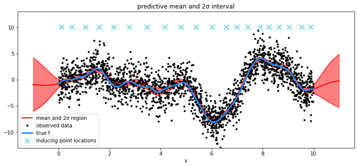
将诱导点位置的优化作为模型的一部分

为了演示目的，我们设置 approx="VFE"。 任何引导点初始化都可以使用任何近似方法完成。

Xu_init = 10 * np.random.rand(20)

with pm.Model() as model:
    ℓ = pm.Gamma("ℓ", alpha=2, beta=1)
    η = pm.HalfCauchy("η", beta=5)

    cov = η**2 * pm.gp.cov.Matern52(1, ℓ)
    gp = pm.gp.MarginalSparse(cov_func=cov, approx="VFE")

    # set flat prior for Xu
    Xu = pm.Flat("Xu", shape=20, testval=Xu_init)

    σ = pm.HalfCauchy("σ", beta=5)
    y_ = gp.marginal_likelihood("y", X=X, Xu=Xu[:, None], y=y, noise=σ)

    mp = pm.find_MAP()

/env/miniconda3/lib/python3.7/site-packages/theano/tensor/basic.py:6611: FutureWarning: Using a non-tuple sequence for multidimensional indexing is deprecated; use `arr[tuple(seq)]` instead of `arr[seq]`. In the future this will be interpreted as an array index, `arr[np.array(seq)]`, which will result either in an error or a different result.
  result[diagonal_slice] = x
/env/miniconda3/lib/python3.7/site-packages/theano/tensor/basic.py:6611: FutureWarning: Using a non-tuple sequence for multidimensional indexing is deprecated; use `arr[tuple(seq)]` instead of `arr[seq]`. In the future this will be interpreted as an array index, `arr[np.array(seq)]`, which will result either in an error or a different result.
  result[diagonal_slice] = x
/env/miniconda3/lib/python3.7/site-packages/theano/tensor/basic.py:6611: FutureWarning: Using a non-tuple sequence for multidimensional indexing is deprecated; use `arr[tuple(seq)]` instead of `arr[seq]`. In the future this will be interpreted as an array index, `arr[np.array(seq)]`, which will result either in an error or a different result.
  result[diagonal_slice] = x

100.00% [118/118 00:01<00:00 logp = -4,301.2, ||grad|| = 2.4568]

/env/miniconda3/lib/python3.7/site-packages/theano/tensor/basic.py:6611: FutureWarning: Using a non-tuple sequence for multidimensional indexing is deprecated; use `arr[tuple(seq)]` instead of `arr[seq]`. In the future this will be interpreted as an array index, `arr[np.array(seq)]`, which will result either in an error or a different result.
  result[diagonal_slice] = x

mu, var = gp.predict(X_new, point=mp, diag=True)
sd = np.sqrt(var)

# draw plot
fig = plt.figure(figsize=(12, 5))
ax = fig.gca()

# plot mean and 2σ intervals
plt.plot(X_new, mu, "r", lw=2, label="mean and 2σ region")
plt.plot(X_new, mu + 2 * sd, "r", lw=1)
plt.plot(X_new, mu - 2 * sd, "r", lw=1)
plt.fill_between(X_new.flatten(), mu - 2 * sd, mu + 2 * sd, color="r", alpha=0.5)

# plot original data and true function
plt.plot(X, y, "ok", ms=3, alpha=1.0, label="observed data")
plt.plot(X, f_true, "dodgerblue", lw=3, label="true f")
Xu = mp["Xu"]
plt.plot(Xu, 10 * np.ones(Xu.shape[0]), "cx", ms=10, label="Inducing point locations")

plt.xlabel("x")
plt.ylim([-13, 13])
plt.title("predictive mean and 2σ interval")
plt.legend();

%load_ext watermark
%watermark -n -u -v -iv -w

pymc3  3.9.0
theano 1.0.4
numpy  1.18.5
last updated: Mon Jun 15 2020 

CPython 3.7.7
IPython 7.15.0
watermark 2.0.2