高斯过程：HSGP参考与第一步#

希尔伯特空间高斯过程近似是一种低秩高斯过程近似方法，特别适用于像PyMC这样的概率编程语言。它使用一组预先计算且固定的基函数来近似高斯过程，这些基函数不依赖于协方差核的形式或其超参数。这是一种参数化近似方法，因此在PyMC中可以通过pm.Data或pm.set_data像线性模型一样进行预测。您不需要定义非参数化高斯过程所依赖的.conditional分布。这使得将HSGP（而不是GP）集成到现有的PyMC模型中更加容易。此外，与其他许多高斯过程近似方法不同，HSGP可以在模型的任何地方使用，并且可以与任何似然函数一起使用。

它也非常快。对于未近似的GP，每个MCMC步骤的计算成本为\(\mathcal{O}(n^3)\)，其中\(n\)是数据点的数量。对于HSGP，计算成本为\(\mathcal{O}(mn + m)\)，其中\(m\)是基向量的数量。需要注意的是，采样速度也很大程度上取决于后验几何形状。

HSGP近似确实有一些限制：

它只能与平稳协方差核一起使用，例如Matern族。HSGP类与任何实现了power_spectral_density方法的Covariance类兼容。对于Periodic协方差，PyMC中有一个特殊情况，由HSGPPeriodic实现。
它在输入维度上扩展性不佳。如果你的高斯过程是基于一维过程（如时间序列）或二维空间点过程，HSGP近似是一个很好的选择。当输入维度大于三时，它可能不是一个高效的选择。
它可能难以应对变化更快的进程。如果你试图建模的过程相对于域的范围变化非常快，HSGP近似可能无法准确表示它。我们将在后面的章节中展示如何设置近似的精度，这涉及到近似的保真度与计算复杂性之间的权衡。
对于较小的数据集，完整未近似的GP可能仍然更高效。

该实现的次要目标是通过模块化方式实现核心计算的可访问实现来实现灵活性。对于基本用法，用户可以使用 .prior 和 .conditional 方法，并将 HSGP 类视为 pm.gp.Latent（未近似的 GP）的直接替代品。更高级的用户可以绕过这些方法，转而使用 .prior_linearized，它将 HSGP 暴露为一个参数化模型。对于包含多个 HSGP 的更复杂模型，用户可以直接使用诸如 pm.gp.hsgp_approx.calc_eigenvalues 和 pm.gp.hsgp_approx.calc_eigenvectors 之类的函数。

参考资料：#

原始参考: Solin & Sarkka, 2019.
概率编程语言中的HSGPs: Riutort-Mayol等, 2020.
HSTPs（学生-t过程）：Sellier & Dellaportas, 2023。
Kronecker HSGPs: Dan 等人, 2022
PyMC 的 HSGP API

示例 1: 基本 HSGP 使用#

我们将使用模拟数据来概述HSGP的使用。如果您对此感兴趣，请参考本节：

看到一个简单的 HSGP 示例。
替换标准GP，即pm.gp.Latent，使用更快的近似方法——只要您使用的是更常见的协方差核之一，如ExpQuad、Matern52或Matern32。
理解何时使用中心化或非中心化的参数化方法。
加性高斯过程的快速示例

import arviz as az
import matplotlib.pyplot as plt
import numpy as np
import preliz as pz
import pymc as pm
import pytensor.tensor as pt

# Sample on the CPU
%env CUDA_VISIBLE_DEVICES=''
# import jax
# import numpyro
# numpyro.set_host_device_count(6)

env: CUDA_VISIBLE_DEVICES=''

az.style.use("arviz-whitegrid")
plt.rcParams["figure.figsize"] = [12, 5]
%config InlineBackend.figure_format = 'retina'
seed = sum(map(ord, "hsgp"))
rng = np.random.default_rng(seed)

模拟数据#

def simulate_1d(x, ell_true, eta_true, sigma_true):
    """Given a domain x, the true values of the lengthscale ell, the
    scale eta, and the noise sigma, simulate a one-dimensional GP
    observed at the given x-locations.
    """

    # Draw one sample from the underlying GP.
    n = len(x)
    cov_func = eta_true**2 * pm.gp.cov.Matern52(1, ell_true)
    gp_true = pm.MvNormal.dist(mu=np.zeros(n), cov=cov_func(x[:, None]))
    f_true = pm.draw(gp_true, draws=1, random_seed=rng)

    # The observed data is the latent function plus a small amount
    # of Gaussian distributed noise.
    noise_dist = pm.Normal.dist(mu=0.0, sigma=sigma_true)
    y_obs = f_true + pm.draw(noise_dist, draws=n, random_seed=rng)
    return y_obs, f_true

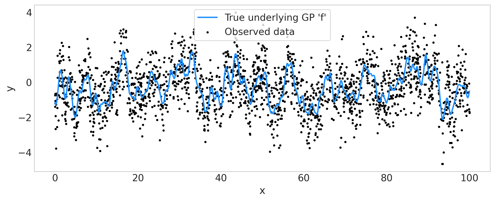
fig = plt.figure(figsize=(10, 4))
ax = fig.gca()

x = 100.0 * np.sort(np.random.rand(2000))
y_obs, f_true = simulate_1d(x=x, ell_true=1.0, eta_true=1.0, sigma_true=1.0)
ax.plot(x, f_true, color="dodgerblue", lw=2, label="True underlying GP 'f'")
ax.scatter(x, y_obs, marker="o", color="black", s=5, label="Observed data")
ax.set_xlabel("x")
ax.set_ylabel("y")
ax.legend(frameon=True)
ax.grid(False)

../_images/1b60fee59767da2f31bbbc437e1c4a5ef4a18065d3c4b6e0bd3fe5d2948523e6.png

定义并拟合HSGP模型#

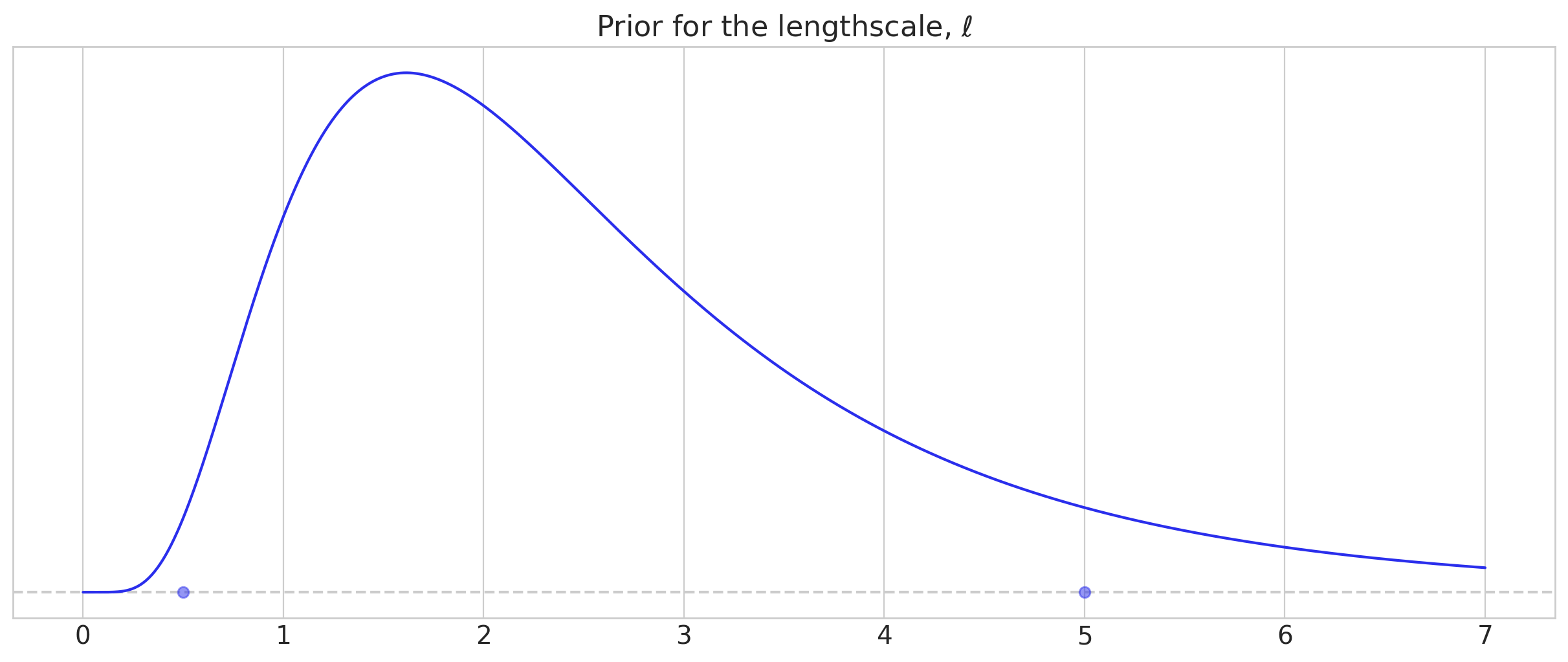
首先我们使用 pz.maxent 来选择长度尺度参数的先验，maxent 返回在区间 [lower, upper] 内具有指定 mass 的最大熵先验。

我们使用对数正态分布来惩罚非常小的长度尺度，同时具有较重的右尾。当来自高斯过程的信号相对于噪声较高时，我们能够使用更具信息量的先验。

lower, upper = 0.5, 5.0
ell_dist, ax = pz.maxent(
    pz.LogNormal(),
    lower=lower,
    upper=upper,
    mass=0.9,
    plot_kwargs={"support": (0, 7), "legend": None},
)

ax.set_title(r"Prior for the lengthscale, $\ell$")

Text(0.5, 1.0, 'Prior for the lengthscale, $\\ell$')

../_images/9b0f0eef0922bb2b4a1fe1dbc44b5cc7b7d570e3dbda1036bbae7bfbec1d7623.png

关于下面的模型代码，有几点需要注意：

近似参数 m 和 c 控制了近似精度与计算复杂度之间的权衡。我们将在后面的部分中看到如何选择这些值。简而言之，选择较大的 m 有助于提高对较小长度尺度和GP需要拟合的其他短距离变化的近似精度。选择较大的 c 有助于提高对较长和较慢变化的近似精度。
我们选择了centered参数化方法，因为真实的潜在高斯过程（GP）受到数据的强烈影响。你可以在这里和这里阅读更多关于centered与non-centered的内容。在HSGP类中，默认是non-centered，这在更常见的、潜在高斯过程（GP）受到观测数据影响较弱的情况下效果更好。

with pm.Model(coords={"basis_coeffs": np.arange(200), "obs_id": np.arange(len(y_obs))}) as model:
    ell = ell_dist.to_pymc("ell")
    eta = pm.Exponential("eta", scale=1.0)
    cov_func = eta**2 * pm.gp.cov.Matern52(input_dim=1, ls=ell)

    # m and c control the fidelity of the approximation
    m, c = 200, 1.5
    parametrization = "centered"
    gp = pm.gp.HSGP(m=[m], c=c, parametrization=parametrization, cov_func=cov_func)
    # Compare to the code for the full, unapproximated GP:
    # gp = pm.gp.Latent(cov_func=cov_func)
    f = gp.prior("f", X=x[:, None], hsgp_coeffs_dims="basis_coeffs", gp_dims="obs_id")

    sigma = pm.Exponential("sigma", scale=1.0)
    pm.Normal("y_obs", mu=f, sigma=sigma, observed=y_obs, dims="obs_id")

    idata = pm.sample()
    idata.extend(pm.sample_posterior_predictive(idata, random_seed=rng))

Auto-assigning NUTS sampler...
Initializing NUTS using jitter+adapt_diag...
Multiprocess sampling (4 chains in 4 jobs)
NUTS: [ell, eta, f_hsgp_coeffs_, sigma]

Sampling 4 chains for 1_000 tune and 1_000 draw iterations (4_000 + 4_000 draws total) took 133 seconds.
Sampling: [y_obs]

az.summary(idata, var_names=["eta", "ell", "sigma"], round_to=2)

	mean	sd	hdi_3%	hdi_97%	ess_bulk	ess_tail	r_hat
eta	0.91	0.08	0.77	1.07	3468.12	3062.29	1.0
ell	0.94	0.10	0.76	1.13	1476.96	2829.41	1.0
sigma	1.01	0.02	0.98	1.04	8891.85	3058.98	1.0

az.plot_trace(
    idata,
    var_names=["eta", "ell", "sigma"],
    lines=[("eta", {}, [1]), ("ell", {}, [1]), ("sigma", {}, [1])],
);

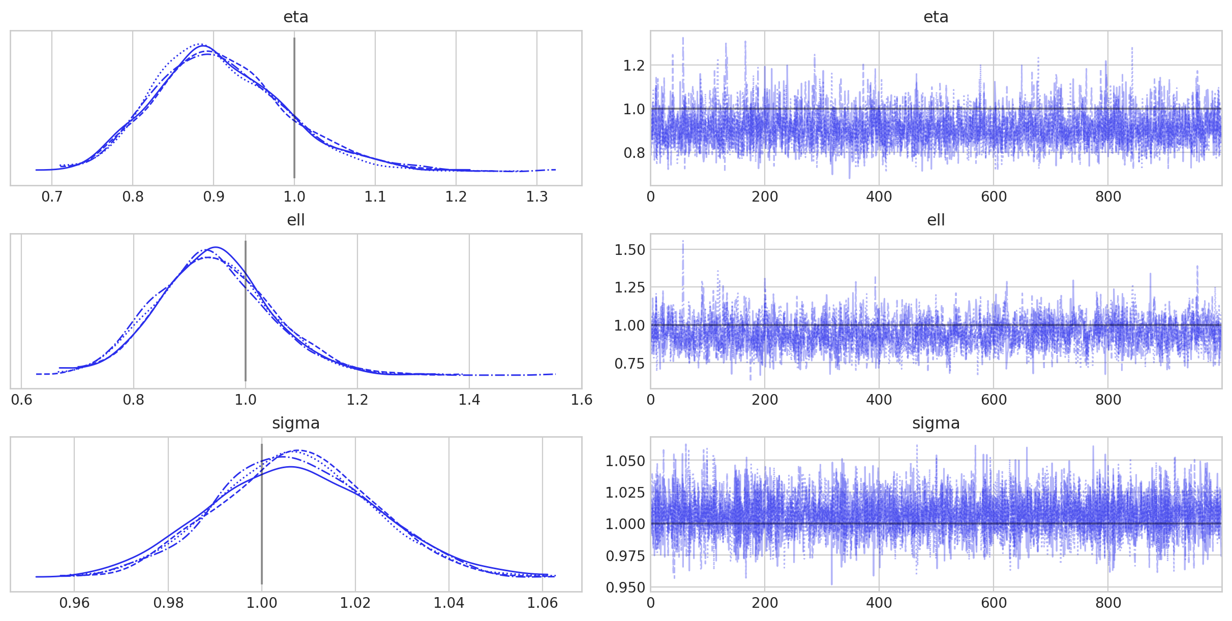
../_images/0dca9024920c020357014464362ea2df18a9540127769cd4dafd72759b60e9d3.png

拟合进行得很顺利，所以我们可以继续绘制推断的高斯过程，以及后验预测样本。

后验预测图#

fig = plt.figure(figsize=(10, 4))
ax = fig.gca()

f = az.extract(idata.posterior.sel(draw=slice(None, None, 10)), var_names="f")
y_preds = az.extract(idata.posterior_predictive.sel(draw=slice(None, None, 10)), var_names="y_obs")

ax.plot(x, y_preds, color="#AAC4E6", alpha=0.02)
ax.plot(x, f, color="#70133A", alpha=0.1)
ax.scatter(x, y_obs, marker="o", color="grey", s=15, label="Observed data")
ax.plot(x, f_true, color="#FBE64D", lw=2, label="True underlying GP 'f'")

ax.set(title="The HSGP Fit", xlabel="x", ylabel="y")
ax.legend(frameon=True, fontsize=11, ncol=2);

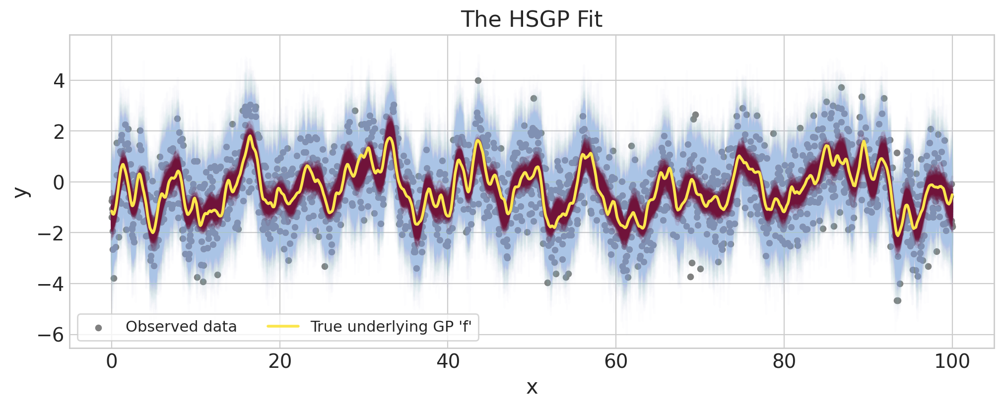
../_images/86132000c64412face7349d5a10fbfd81cc15587b64e3bf8eaa5117f7112ddbc.png

推断出的底层GP（在波尔多）准确匹配真实的底层GP（在黄色）。我们还看到后验预测样本（在浅蓝色）非常吻合观测数据。

加性高斯过程

HSGP 兼容加性协方差，而不是定义两个完全独立的 HSGP。

与其直接构造并添加它们，计算两个HSGP之和可以更高效地通过首先计算它们功率谱密度的和，然后从组合的功率谱密度创建一个单一的GP来实现。这减少了未知参数的数量，因为两个GP可以共享相同的基集。

这个代码看起来类似于：

cov1 = eta1**2 * pm.gp.cov.ExpQuad(input_dim, ls=ell1)
cov2 = eta2**2 * pm.gp.cov.Matern32(input_dim, ls=ell2)
cov = cov1 + cov2

gp = pm.gp.HSGP(m=[m], c=c, cov_func=cov_func)

选择HSGP近似参数，`m`，`L`，和`c`#

在使用HSGP拟合模型之前，您必须选择m和c或L。m是基向量的数量。回想一下，HSGP近似的计算复杂度是\(\mathcal{O}(mn + m)\)，其中\(n\)是数据点的数量。

这个选择是三个关注点之间的平衡：

近似的准确性。
减少计算负担。
需要进行预测或预报的X位置。

在本节末尾，我们将给出Ruitort-Mayol等人提出的经验法则。理解如何选择这些参数的最佳方法是理解m、c和L之间的关系，这需要进一步了解近似方法在底层的工作原理。

如何`L`和`c`影响基础#

非技术性地讲，HSGP将GP先验近似为正弦波的线性组合。线性组合的系数是独立同分布的正态随机变量，其标准差取决于GP超参数（对于Matern族，这些超参数是幅度和长度尺度）。

为了了解这一点，我们将绘制一些\(m=3\)和\(m=5\)基向量的图，并仔细观察它们在定义域边界处的行为。请注意，我们必须首先将x数据居中，然后根据居中的数据选择L。值得一提的是，我们绘制的基向量不依赖于协方差核的选择，也不依赖于协方差函数可能具有的任何未知参数。

# Our data goes from x=-5 to x=5
x = np.linspace(-5, 5, 1000)

# (plotting code)
fig, axs = plt.subplots(1, 3, figsize=(14, 4), sharey=True, constrained_layout=True)

ylim = 0.55
axs[0].set_ylim([-ylim, ylim])
axs[1].set_yticks([])
axs[1].set_xlabel("xs (mean subtracted x)")
axs[2].set_yticks([])

# change L as we create the basis vectors
L_options = [5.0, 6.0, 20.0]
m_options = [3, 3, 5]
for i, ax in enumerate(axs.flatten()):
    L = L_options[i]
    m = m_options[i]

    eigvals = pm.gp.hsgp_approx.calc_eigenvalues(pt.as_tensor([L]), [m])
    phi = pm.gp.hsgp_approx.calc_eigenvectors(
        x[:, None],
        pt.as_tensor([L]),
        eigvals,
        [m],
    ).eval()

    for j in range(phi.shape[1]):
        ax.plot(x, phi[:, j])

    ax.set_xticks(np.arange(-5, 6, 5))

    S = 5.0
    c = L / S
    ax.text(-4.9, -0.45, f"L = {L}\nc = {c}", fontsize=15)
    ax.set(title=f"{m} basis functions")

plt.suptitle("The effect of changing $L$ on the HSGP basis vectors", fontsize=18);

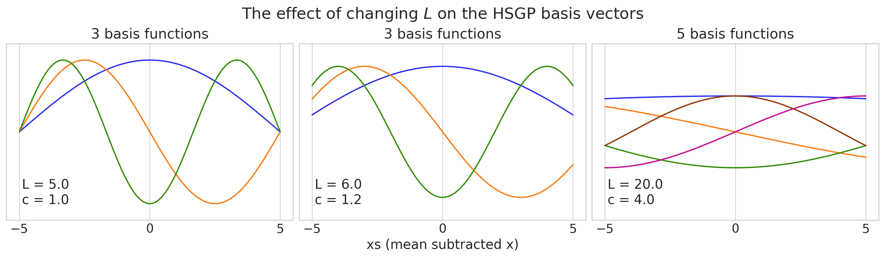
../_images/8544ed194396b7fcbc67c491793c17d5fd5f2d30b72ea52996f584b067e59cfe.png

第一个和中间的面板有3个基函数，最右边的有5个。

请注意，L 和 m 都被指定为列表，以允许按输入维度设置 L 和 m。在这个例子中，这两个都是只有一个元素的列表，因为我们的例子是在一个一维的、类似时间序列的上下文中。在继续之前，定义 \(S\) 为居中数据的半范围，或从中点 \(x=0\) 到边缘 \(x=5\) 的距离，会很有帮助。在这个例子中，每个绘图面板的 \(S=5\)。然后，我们可以定义 \(c\)，使得它与 \(S\) 和 \(L\) 相关，

\[ L = c \cdot S \,. \]

通常通过选择 \(c\) 来设置 \(L\) 更容易，\(c\) 作为 \(S\) 的乘数。

在最左边的图中，我们选择了 \(L=S=5\)，这正好位于我们的 x 位置的边缘。对于任何 \(m\)，所有的基向量都被迫在边缘处收缩到零，即在 \(x=-5\) 和 \(x=5\) 处。这意味着 HSGP 近似在接近 \(x=-5\) 和 \(x=5\) 时会变得较差。这种变差的快慢取决于长度尺度。较大的长度尺度需要较大的 \(L\) 和 \(c\) 值，而较小的长度尺度则会减弱这个问题。Ruitort-Mayol 等人建议使用 1.2 作为最小值。这种选择对基向量的影响显示在中间面板中。特别是，我们现在可以看到基向量不会被迫收缩到零。

右侧面板展示了选择较大的 \(L\) 或设置 \(c=4\) 的效果。较大的 \(L\) 或 \(c\) 值使得边界条件问题减少，并且需要准确近似具有较长长度尺度的GP。您还需要考虑预测将在何处进行。除了观测到的 \(x\) 值的位置外，新的 \(x\) 位置也需要远离由边界条件引起的“收缩”。随着我们增加 \(L\) 或 \(c\)，基函数的周期也会增加。这意味着我们需要增加 \(m\)，即基向量的数量，以进行补偿，如果我们希望近似具有较小长度尺度的GP。

当\(L\)或\(c\)较大时，第一个特征向量可能会变得非常平坦，以至于在模型中与截距部分或完全无法识别。最右边的面板就是一个例子（见蓝色基向量）。在这些情况下，丢弃第一个特征向量对采样非常有利。PyMC中的HSGP和HSGPPeriodic类都有drop_first选项来实现这一点，或者如果你使用.prior_linearized，你可以自己控制这一点。如果采样器出现问题，请务必检查基向量。

总结：

增加 \(m\) 有助于 HSGP 近似具有较小长度尺度的 GP，但会增加计算复杂度。
增加 \(c\) 或 \(L\) 有助于 HSGP 近似具有较大长度尺度的 GP，但可能需要增加 \(m\) 以补偿在较小长度尺度上的保真度损失。
在选择\(m\)、\(c\)或\(L\)时，重要的是考虑你需要进行预测的位置，以确保它们也不受边界条件的影响。
第一个基向量可能无法识别与截距，特别是在 \(L\) 或 \(c\) 较大时。

选择\(m\)和\(c\)的启发式方法#

在实践中，您需要从数据中推断出长度尺度，因此HSGP需要在代表您选择的先验的长度尺度范围内近似一个GP。您需要选择\(c\)足够大以处理您可能拟合的最大长度尺度，并且还需要选择\(m\)足够大以适应最小的长度尺度。

Ruitort-Mayol 等人提供了一些方便的经验法则，用于在给定的 \(m\) 和 \(c\) 值下准确再现的长度尺度范围。下面，我们提供了一个函数，该函数使用他们的经验法则来推荐最小 \(m\) 和 \(c\) 值。请注意，这些推荐是基于一维高斯过程的。

例如，如果你使用的是 Matern52 协方差，并且你的数据范围从 \(x=-5\) 到 \(x=95\)，而你的长度尺度先验主要在 \(\ell=1\) 到 \(\ell=50\) 之间，那么推荐的最小值是 \(m=543\) 和 \(c=3.7\)，如下所示：

m, c = pm.gp.hsgp_approx.approx_hsgp_hyperparams(
    x_range=[-5, 95], lengthscale_range=[1, 50], cov_func="matern52"
)

print("Recommended smallest number of basis vectors (m):", m)
print("Recommended smallest scaling factor (c):", np.round(c, 1))

Recommended smallest number of basis vectors (m): 543
Recommended smallest scaling factor (c): 4.1

HSGP近似Gram矩阵#

由于以下几个原因，您可能无法依赖这些启发式方法。您可能使用了不同于ExpQuad、Matern52或Matern32的协方差函数。此外，它们仅针对一维高斯过程定义。另一种检查HSGP保真度的方法是直接比较未近似的Gram矩阵（Gram矩阵是在输入X上计算协方差函数后得到的矩阵），\(\mathbf{K}\)，与HSGP近似结果得到的矩阵，

\[ \tilde{\mathbf{K}} = \Phi \Delta \Phi^T \,, \]

其中\(\Phi\)是我们用作基的特征向量矩阵（之前绘制过），而\(\Delta\)在特征值上沿对角线计算了光谱密度。下面我们展示了一个二维输入网格X的示例。需要注意的是，HSGP近似要求我们对输入X数据进行中心化处理，这是通过将X转换为Xs在下面的代码中完成的。我们绘制了不同\(L\)和\(c\)值的近似Gram矩阵，以观察在给定的X位置和长度尺度选择下，近似何时开始退化。

## Define the X locations and calculate the Gram matrix from a given covariance function
x1, x2 = np.meshgrid(np.linspace(0, 10, 50), np.linspace(0, 10, 4))
X = np.vstack((x2.flatten(), x1.flatten())).T

# X is two dimensional, so we set input_dim=2
chosen_ell = 3.0
cov_func = pm.gp.cov.ExpQuad(input_dim=2, ls=chosen_ell)
K = cov_func(X).eval()

## Calculate the HSGP approximate Gram matrix
# Center or "scale" X so we can work with Xs (important)
X_center = (np.max(X, axis=0) + np.min(X, axis=0)) / 2.0
Xs = X - X_center

# Calculate L given Xs and c
m, c = [20, 20], 2.0
L = pm.gp.hsgp_approx.set_boundary(Xs, c)

def calculate_Kapprox(Xs, L, m):
    # Calculate Phi and the diagonal matrix of power spectral densities
    eigvals = pm.gp.hsgp_approx.calc_eigenvalues(L, m)
    phi = pm.gp.hsgp_approx.calc_eigenvectors(Xs, L, eigvals, m)
    omega = pt.sqrt(eigvals)
    psd = cov_func.power_spectral_density(omega)
    return (phi @ pt.diag(psd) @ phi.T).eval()

fig, axs = plt.subplots(2, 4, figsize=(14, 7), sharey=True)

axs[0, 0].imshow(K, cmap="inferno", vmin=0, vmax=1)
axs[0, 0].set(xlabel="x1", ylabel="x2", title=f"True Gram matrix\nTrue $\\ell$ = {chosen_ell}")
axs[1, 0].axis("off")
im_kwargs = {
    "cmap": "inferno",
    "vmin": 0,
    "vmax": 1,
    "interpolation": "none",
}

## column 1
m, c = [30, 30], 5.0
L = pm.gp.hsgp_approx.set_boundary(Xs, c)
K_approx = calculate_Kapprox(Xs, L, m)
axs[0, 1].imshow(K_approx, **im_kwargs)
axs[0, 1].set_title(f"m = {m}, c = {c}")

m, c = [30, 30], 1.2
L = pm.gp.hsgp_approx.set_boundary(Xs, c)
K_approx = calculate_Kapprox(Xs, L, m)
axs[1, 1].imshow(K_approx, **im_kwargs)
axs[1, 1].set(xlabel="x1", ylabel="x2", title=f"m = {m}, c = {c}")

## column 2
m, c = [15, 15], 5.0
L = pm.gp.hsgp_approx.set_boundary(Xs, c)
K_approx = calculate_Kapprox(Xs, L, m)
axs[0, 2].imshow(K_approx, **im_kwargs)
axs[0, 2].set_title(f"m = {m}, c = {c}")

m, c = [15, 15], 1.2
L = pm.gp.hsgp_approx.set_boundary(Xs, c)
K_approx = calculate_Kapprox(Xs, L, m)
axs[1, 2].imshow(K_approx, **im_kwargs)
axs[1, 2].set_title(f"m = {m}, c = {c}")

## column 3
m, c = [2, 2], 5.0
L = pm.gp.hsgp_approx.set_boundary(Xs, c)
K_approx = calculate_Kapprox(Xs, L, m)
axs[0, 3].imshow(K_approx, **im_kwargs)
axs[0, 3].set_title(f"m = {m}, c = {c}")

m, c = [2, 2], 1.2
L = pm.gp.hsgp_approx.set_boundary(Xs, c)
K_approx = calculate_Kapprox(Xs, L, m)
axs[1, 3].imshow(K_approx, **im_kwargs)
axs[1, 3].set_title(f"m = {m}, c = {c}")

for ax in axs.flatten():
    ax.grid(False)
plt.tight_layout();

/tmp/ipykernel_21840/3948114812.py:54: UserWarning: The figure layout has changed to tight
  plt.tight_layout();

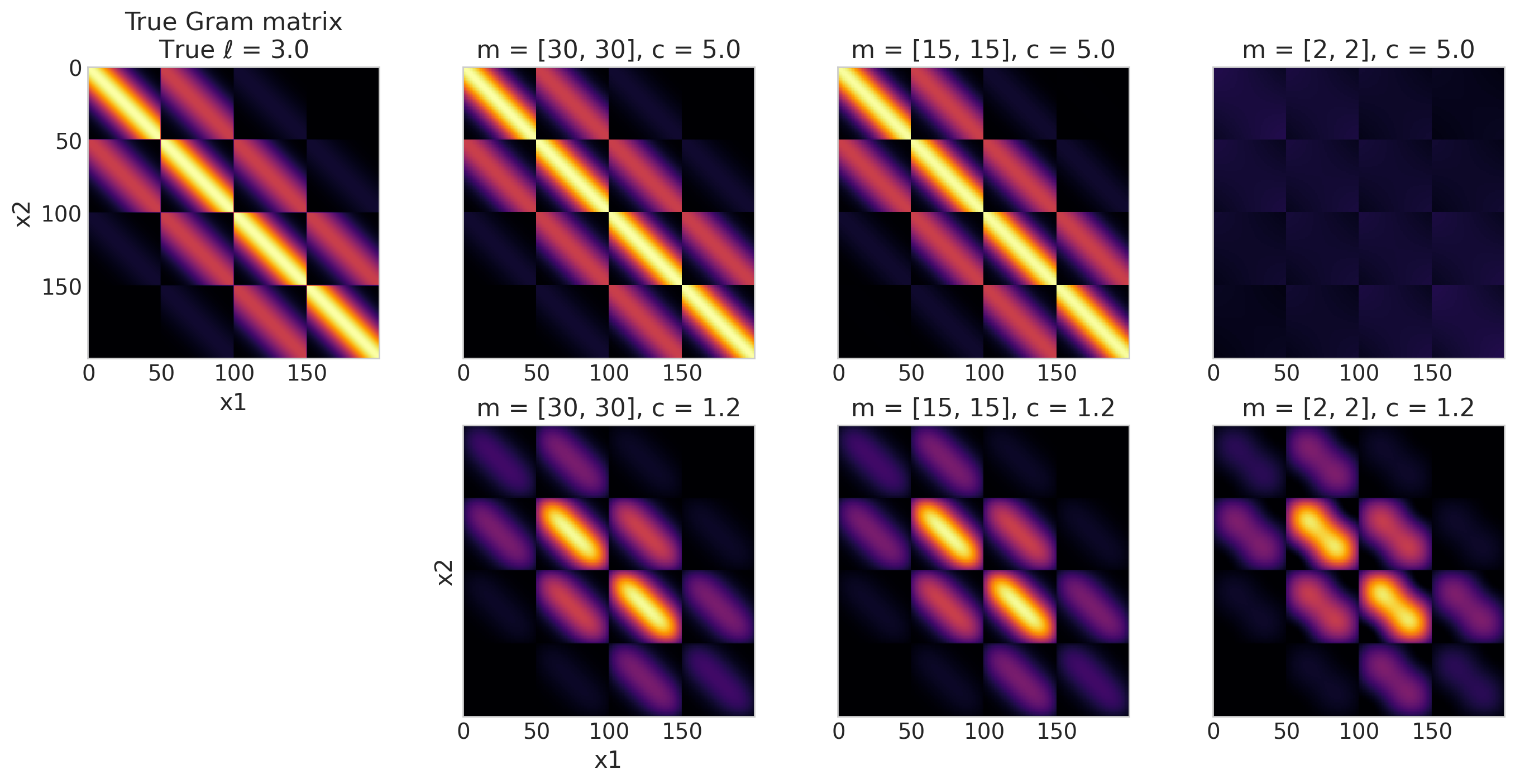
../_images/58565f84917ea27e314c3080fbadb56c7d7fc95b6ef906c37941e6540b125abb.png

上面的图比较了近似的Gram矩阵与左上角未近似的Gram矩阵。目标是将近似的Gram矩阵与真实的Gram矩阵（左上角）进行比较。定性地，它们看起来越相似，近似效果越好。此外，这些结果仅与由X和所选长度尺度定义的特定领域相关，\(\ell = 3\)——仅仅因为对于\(\ell = 3\)看起来不错，并不意味着对于例如\(\ell = 10\)也会看起来不错。

我们可以得出一些结论：

对于两个面板，当 \(m = 15\) 或 \(m = 30\)，并且 \(c=5.0\) 时，近似看起来在视觉上效果良好。其余部分显示出与未近似的Gram矩阵有明显的差异。
\(c=1.2\) 通常太小，无论 \(m\) 如何。
也许令人惊讶的是，\(m=[2, 2]\)，\(c=1.2\) 的近似看起来比 \(m=[2, 2]\)，\(c=5\) 的更好。正如我们之前展示的，当我们“拉伸”特征向量基以填充比我们的 X（通过倍数 \(c\) 扩大）更大的域时，我们可能会在较小的长度尺度上失去保真度。换句话说，在第二种情况下，\(m\) 对于 \(c\) 的值来说太小了。这就是为什么第一个选项看起来更好的原因。
第二行（\(c=1.2\)）并没有随着\(m\)的增加而真正改善。这是因为\(m\)已经足够捕捉较小的长度尺度，但\(c\)总是太小，无法捕捉较大的长度尺度。
另一方面，第一行显示对于较大的长度尺度，\(c=5\)已经足够好，并且一旦我们达到\(m=15\)，我们也能够捕捉到较小的长度尺度。

对于您的特定情况，您需要在不同的长度尺度范围内进行实验，并量化可以接受的近似误差。通常，在原型模型时，您可以使用较低保真度的HSGP近似来加快采样速度。然后，一旦您了解了相关长度尺度的范围，您就可以调整正确的\(m\)和\(L\)（或\(c\)）值。

请注意，也有可能遇到低保真度HSGP近似比高保真度HSGP近似更简洁的情况。低保真度HSGP近似对于某些未知函数仍然是一个有效的先验，尽管有些牵强。这是否重要将取决于您的上下文。

示例 2：将 HSGPs 作为参数化线性模型使用#

HSGP近似的主要优点之一是能够将其集成到现有模型中，特别是在采样后需要在新的x位置进行预测的情况下。与PyMC中的其他GP实现不同，您可以绕过.prior和.conditional API，而是使用HSGP.prior_linearized，这允许您使用pm.Data和pm.set_data来进行预测。

如果您对此部分感兴趣，请参考：

查看一个二维或空间的高斯过程样例，模型中包含其他预测因子。
在较大的 PyMC 模型中使用 HSGPs 进行预测。
将您的 HSGP 近似转换为 HSTP 近似，或转换为 TP 近似，或学生-t 过程的近似。

数据生成#

def simulate_2d(
    beta0_true,
    beta1_true,
    ell_true,
    eta_true,
    sigma_true,
):
    # Create the 2d X locations
    from scipy.stats import qmc

    sampler = qmc.Sobol(d=2, scramble=False, optimization="lloyd")
    X = 20 * sampler.random_base2(m=11) - 10.0

    # add the fixed effect at specific intervals
    ix = 1.0 * (np.abs(X[:, 0] // 5) == 1)
    X = np.hstack((X, ix[:, None]))

    # Draw one sample from the underlying GP
    n = X.shape[0]
    cov_func = eta_true**2 * pm.gp.cov.Matern52(3, ell_true, active_dims=[0, 1])
    gp_true = pm.MvNormal.dist(mu=np.zeros(n), cov=cov_func(X))
    f_true = pm.draw(gp_true, draws=1, random_seed=rng)

    # Add the fixed effects
    mu = beta0_true + beta1_true * X[:, 2] + f_true

    # The observed data is the latent function plus a small amount
    # of Gaussian distributed noise.
    noise_dist = pm.Normal.dist(mu=0.0, sigma=sigma_true)
    y_obs = mu + pm.draw(noise_dist, draws=n, random_seed=rng)
    return y_obs, f_true, mu, X

y_obs, f_true, mu, X = simulate_2d(
    beta0_true=3.0,
    beta1_true=2.0,
    ell_true=1.0,
    eta_true=1.0,
    sigma_true=0.75,
)

# Split into train and test sets
ix_tr = (X[:, 1] < 2) | (X[:, 1] > 4)
ix_te = (X[:, 1] > 2) & (X[:, 1] < 4)

X_tr, X_te = X[ix_tr, :], X[ix_te, :]
y_tr, y_te = y_obs[ix_tr], y_obs[ix_te]

fig = plt.figure(figsize=(13, 4))
plt.subplots_adjust(wspace=0.02)

ax1 = plt.subplot(131)
ax1.scatter(X_tr[:, 0], X_tr[:, 1], c=mu[ix_tr] - f_true[ix_tr])
ax1.set_title("$\\beta_0 + \\beta_1 X$")
ax1.set_ylabel("$x_1$", rotation=0)

ax2 = plt.subplot(132)
ax2.scatter(X_tr[:, 0], X_tr[:, 1], c=f_true[ix_tr])
ax2.set_title("The spatial GP, $f$")
ax2.set_yticks([])
ax2.set_xlabel("$x_0$")

ax3 = plt.subplot(133)
im = ax3.scatter(X_tr[:, 0], X_tr[:, 1], c=y_obs[ix_tr])
ax3.set_title("The observed data, $y$")
ax3.set_yticks([])

fig.colorbar(im, ax=[ax1, ax2, ax3]);

/tmp/ipykernel_21840/2813859405.py:2: UserWarning: This figure was using a layout engine that is incompatible with subplots_adjust and/or tight_layout; not calling subplots_adjust.
  plt.subplots_adjust(wspace=0.02)

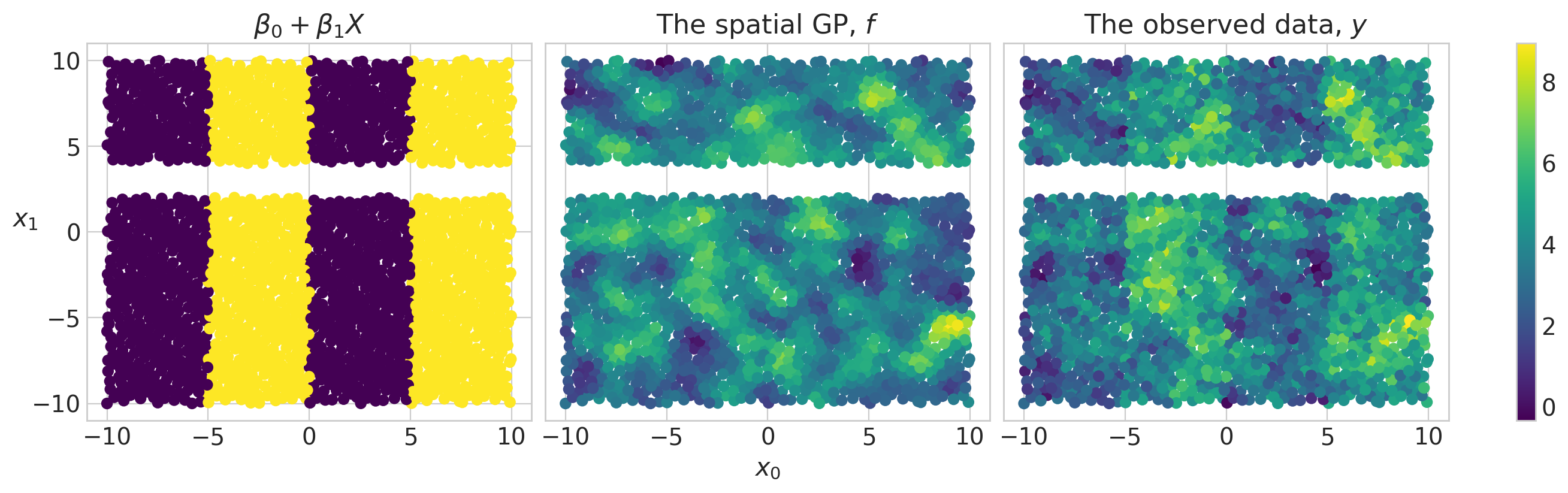
../_images/be5c621c8d7e8af9d2980e3b20045dafdf9430499d83069236a396d582954d54.png

正如预期的那样，我们清楚地看到测试集位于\(2 < x1 < 4\)的区域内。

这里是与我们生成场景相对应的模型结构。下面我们描述其主要组件。

模型结构#

with pm.Model() as model:
    # Set mutable data
    X_gp = pm.Data("X_gp", X_tr[:, :2])
    X_fe = pm.Data("X_fe", X_tr[:, 2])

    # Priors on regression coefficients
    beta = pm.Normal("beta", mu=0.0, sigma=10.0, shape=2)

    # Prior on the HSGP
    eta = pm.Exponential("eta", scale=2.0)
    ell_params = pm.find_constrained_prior(
        pm.Lognormal, lower=0.5, upper=5.0, mass=0.9, init_guess={"mu": 1.0, "sigma": 1.0}
    )
    ell = pm.Lognormal("ell", **ell_params)
    cov_func = eta**2 * pm.gp.cov.Matern52(input_dim=2, ls=ell)

    # m and c control the fidelity of the approximation
    m0, m1, c = 30, 30, 2.0
    gp = pm.gp.HSGP(m=[m0, m1], c=c, cov_func=cov_func)

    phi, sqrt_psd = gp.prior_linearized(X=X_gp)

    basis_coeffs = pm.Normal("basis_coeffs", size=gp.n_basis_vectors)
    f = pm.Deterministic("f", phi @ (basis_coeffs * sqrt_psd))

    mu = pm.Deterministic("mu", beta[0] + beta[1] * X_fe + f)

    sigma = pm.Exponential("sigma", scale=2.0)
    pm.Normal("y_obs", mu=mu, sigma=sigma, observed=y_tr, shape=X_gp.shape[0])

    idata = pm.sample_prior_predictive(random_seed=rng)

pm.model_to_graphviz(model)

Sampling: [basis_coeffs, beta, ell, eta, sigma, y_obs]

../_images/595ea2469e326955081720a549ceeff00466e432bfb8b1749fad94f7c64a33e2.svg

在采样和查看结果之前，上述模型中有几点需要注意。

设置系数，中心化和非中心化#

首先，prior_linearized 返回特征向量基，phi，以及特征值处的功率谱平方根，sqrt_psd。你需要从这些构造 HSGP 近似。以下是相关代码行，展示了中心化和非中心化的参数化。

phi, sqrt_psd = gp.prior_linearized(X=X)

## non-centered
basis_coeffs= pm.Normal("basis_coeffs", size=gp.n_basis_vectors)
f = pm.Deterministic("f", phi @ (beta * sqrt_psd)) 

## centered
basis_coeffs= pm.Normal("basis_coeffs", sigma=sqrt_psd, size=gp.n_basis_vectors)
f = pm.Deterministic("f", phi @ beta) 

请确保使用HSGP对象的n_basis_vectors属性（或phi的列数）设置basis_coeffs的大小，\(m^* = \prod_i m_i\)。在上面的示例中，\(m^* = 30 \cdot 30 = 900\)，并且是近似中使用的基向量的总数。

近似一个TP而不是一个GP#

我们可以稍微修改上面的代码来获得一个学生-t过程，

nu = pm.Gamma("nu", alpha=2, beta=0.1)
basis_coeffs= pm.StudentT("basis_coeffs", nu=nu, size=gp.n_basis_vectors)
f = pm.Deterministic("f", phi @ (beta * sqrt_psd)) 

我们使用一个\(\text{Gamma}(\alpha=2, \beta=0.1)\)先验分布来表示\(\nu\)，这使得大约有50%的概率\(\nu > 30\)，即在Student-T分布大致变得与高斯分布无法区分的地方。更多信息请参见此链接。

结果#

现在，让我们对模型进行采样并快速检查结果：

with model:
    idata.extend(pm.sample(nuts_sampler="numpyro", random_seed=rng))

2024-08-17 10:55:34.390278: E external/xla/xla/service/slow_operation_alarm.cc:65] Constant folding an instruction is taking > 1s:

  %reduce = f64[4,1000,900,1]{3,2,1,0} reduce(f64[4,1000,1,900,1]{4,3,2,1,0} %broadcast.8, f64[] %constant.14), dimensions={2}, to_apply=%region_1.45, metadata={op_name="jit(process_fn)/jit(main)/reduce_prod[axes=(2,)]" source_file="/tmp/tmp7cn2oyvr" source_line=33}

This isn't necessarily a bug; constant-folding is inherently a trade-off between compilation time and speed at runtime. XLA has some guards that attempt to keep constant folding from taking too long, but fundamentally you'll always be able to come up with an input program that takes a long time.

If you'd like to file a bug, run with envvar XLA_FLAGS=--xla_dump_to=/tmp/foo and attach the results.
2024-08-17 10:55:36.431977: E external/xla/xla/service/slow_operation_alarm.cc:133] The operation took 3.041937496s
Constant folding an instruction is taking > 1s:

  %reduce = f64[4,1000,900,1]{3,2,1,0} reduce(f64[4,1000,1,900,1]{4,3,2,1,0} %broadcast.8, f64[] %constant.14), dimensions={2}, to_apply=%region_1.45, metadata={op_name="jit(process_fn)/jit(main)/reduce_prod[axes=(2,)]" source_file="/tmp/tmp7cn2oyvr" source_line=33}

This isn't necessarily a bug; constant-folding is inherently a trade-off between compilation time and speed at runtime. XLA has some guards that attempt to keep constant folding from taking too long, but fundamentally you'll always be able to come up with an input program that takes a long time.

If you'd like to file a bug, run with envvar XLA_FLAGS=--xla_dump_to=/tmp/foo and attach the results.

idata.sample_stats.diverging.sum().data

array(0)

var_names = [var.name for var in model.free_RVs if var.size.eval() <= 2]
az.summary(idata, var_names=var_names, round_to=2)

	mean	sd	hdi_3%	hdi_97%	ess_bulk	ess_tail	r_hat
beta[0]	2.97	0.12	2.76	3.19	6895.09	2705.11	1.0
beta[1]	1.97	0.11	1.76	2.17	8498.54	2687.87	1.0
eta	1.06	0.06	0.95	1.17	1601.09	2599.12	1.0
ell	0.80	0.09	0.64	0.97	2089.67	2878.43	1.0
sigma	0.81	0.01	0.79	0.84	5583.59	3112.06	1.0

az.plot_trace(
    idata,
    var_names=var_names,
    lines=[("beta", {}, [3, 2]), ("ell", {}, [1]), ("eta", {}, [1]), ("sigma", {}, [0.75])],
);

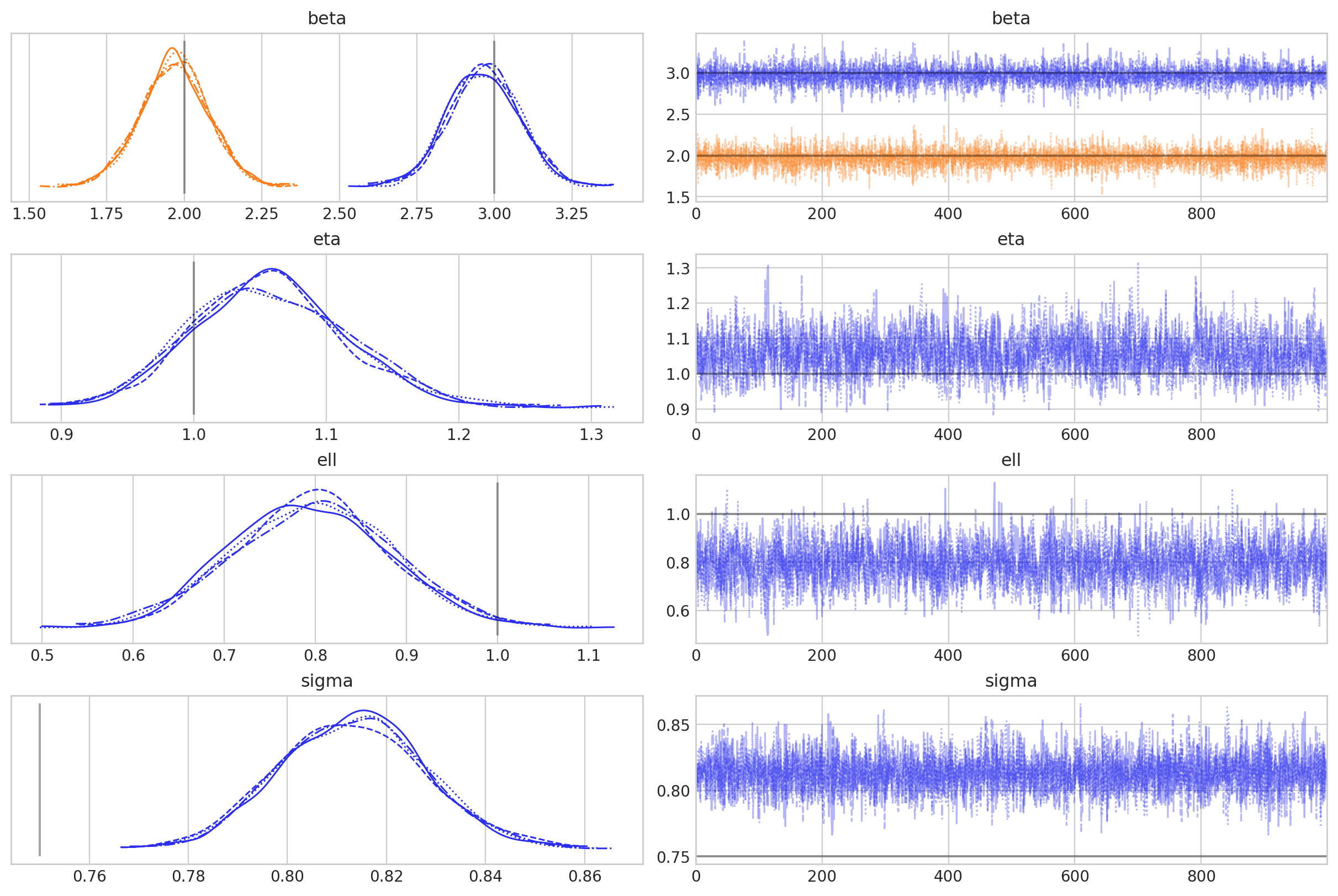
../_images/ec5444e06f838bf3c1cab18954b7dd9fa6442927b5d17bfea28eff4a13ef1069.png

采样进行得很顺利，但有趣的是，我们似乎在后验中对sigma存在偏差。这不是本笔记本的重点，但在实际用例中深入探讨这一点会很有趣。

样本外预测#

然后，我们可以直接使用 pm.set_data 在新点上进行预测。我们将在下面的图中展示拟合结果和预测结果。

with model:
    pm.set_data({"X_gp": X[:, :2], "X_fe": X[:, 2]})

    idata_thinned = idata.sel(draw=slice(None, None, 10))
    idata.extend(
        pm.sample_posterior_predictive(idata_thinned, var_names=["f", "mu"], random_seed=rng)
    )

Sampling: []

pm.model_to_graphviz(model)

../_images/8c1e08d8e5e9eb9268fc2c6566e6bc34af6706106117fbd3ba7174816c39b22c.svg

fig = plt.figure(figsize=(13, 4))
plt.subplots_adjust(wspace=0.02)

ax1 = plt.subplot(131)
ax1.scatter(X[:, 0], X[:, 1], c=f_true)
ax1.set_title("True underlying GP")
ax1.set_xlabel("$x_0$")
ax1.set_ylabel("$x_1$", rotation=0)

ax2 = plt.subplot(132)
f_sd = az.extract(idata.posterior_predictive, var_names="f").std(dim="sample")
ax2.scatter(X[:, 0], X[:, 1], c=f_sd)
ax2.set_title("Std. dev. of the inferred GP")
ax2.set_yticks([])
ax2.set_xlabel("$x_0$")

ax3 = plt.subplot(133)
f_mu = az.extract(idata.posterior_predictive, var_names="f").mean(dim="sample")
im = ax3.scatter(X[:, 0], X[:, 1], c=f_mu)
ax3.set_title("Mean of the inferred GP")
ax3.set_yticks([])
ax3.set_xlabel("$x_0$")

fig.colorbar(im, ax=[ax1, ax2, ax3]);

/tmp/ipykernel_21840/3852779046.py:2: UserWarning: This figure was using a layout engine that is incompatible with subplots_adjust and/or tight_layout; not calling subplots_adjust.
  plt.subplots_adjust(wspace=0.02)

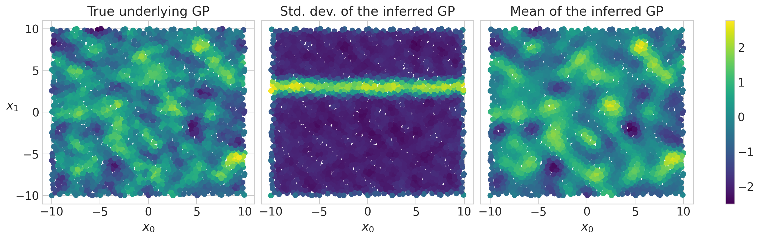
../_images/f54096a5a7e5f43ca58a473a20c382511113a8b74f421d9a924c8291a7c9c306.png

采样诊断结果看起来都很好，我们可以看到潜在的GP被很好地推断出来了。我们还可以在中面板中看到训练数据之外的不确定性增加，表现为中间的水平条纹，显示了此处推断的GP标准偏差的增加。

作者#

由 Bill Engels 和 Alexandre Andorra 于2024年创建（pymc-examples#647）
使用 pz.maxent 代替 pm.find_constrained_prior，并添加随机种子。Osvaldo Martin。2024年8月

水印#

%load_ext watermark
%watermark -n -u -v -iv -w -p xarray

Last updated: Sat Aug 17 2024

Python implementation: CPython
Python version       : 3.11.5
IPython version      : 8.16.1

xarray: 2023.10.1

pytensor  : 2.25.2
matplotlib: 3.8.4
pymc      : 5.16.2+20.g747fda319
numpy     : 1.24.4
preliz    : 0.9.0
arviz     : 0.19.0.dev0

Watermark: 2.4.3

许可证声明#

本示例库中的所有笔记本均在MIT许可证下提供，该许可证允许修改和重新分发，前提是保留版权和许可证声明。

引用 PyMC 示例#

要引用此笔记本，请使用Zenodo为pymc-examples仓库提供的DOI。

重要

许多笔记本是从其他来源改编的：博客、书籍……在这种情况下，您应该引用原始来源。

同时记得引用代码中使用的相关库。

这是一个BibTeX的引用模板：

@incollection{citekey,
  author    = "<notebook authors, see above>",
  title     = "<notebook title>",
  editor    = "PyMC Team",
  booktitle = "PyMC examples",
  doi       = "10.5281/zenodo.5654871"
}

渲染后可能看起来像：

分类

标签

高斯过程：HSGP参考与第一步#

参考资料：#

示例 1: 基本 HSGP 使用#

模拟数据#

定义并拟合HSGP模型#

后验预测图#

选择HSGP近似参数，`m`，`L`，和`c`#

如何`L`和`c`影响基础#

选择\(m\)和\(c\)的启发式方法#

HSGP近似Gram矩阵#

示例 2：将 HSGPs 作为参数化线性模型使用#

数据生成#

模型结构#

设置系数，中心化和非中心化#

近似一个TP而不是一个GP#

结果#

样本外预测#

作者#

水印#

许可证声明#

引用 PyMC 示例#

分类

标签

高斯过程：HSGP参考与第一步#

参考资料：#

示例 1: 基本 HSGP 使用#

模拟数据#

定义并拟合HSGP模型#

后验预测图#

选择HSGP近似参数，m，L，和c#

如何L和c影响基础#

选择\(m\)和\(c\)的启发式方法#

HSGP近似Gram矩阵#

示例 2：将 HSGPs 作为参数化线性模型使用#

数据生成#

模型结构#

设置系数，中心化和非中心化#

近似一个TP而不是一个GP#

结果#

样本外预测#

作者#

水印#

许可证声明#

引用 PyMC 示例#

选择HSGP近似参数，`m`，`L`，和`c`#

如何`L`和`c`影响基础#