


多输出高斯过程:使用哈达玛积的协区域化模型#
本笔记本展示了如何使用Coregion核与输入核之间的哈达玛积来实现固有共区域化模型(ICM)和线性共区域化模型(LCM)。多输出高斯过程在这篇论文中由Bonilla 等人 [2007]讨论。有关ICM和LCM的更多信息,请查看Mauricio Alvarez关于多输出高斯过程的演讲,以及他的幻灯片,最后一页有更多参考资料。
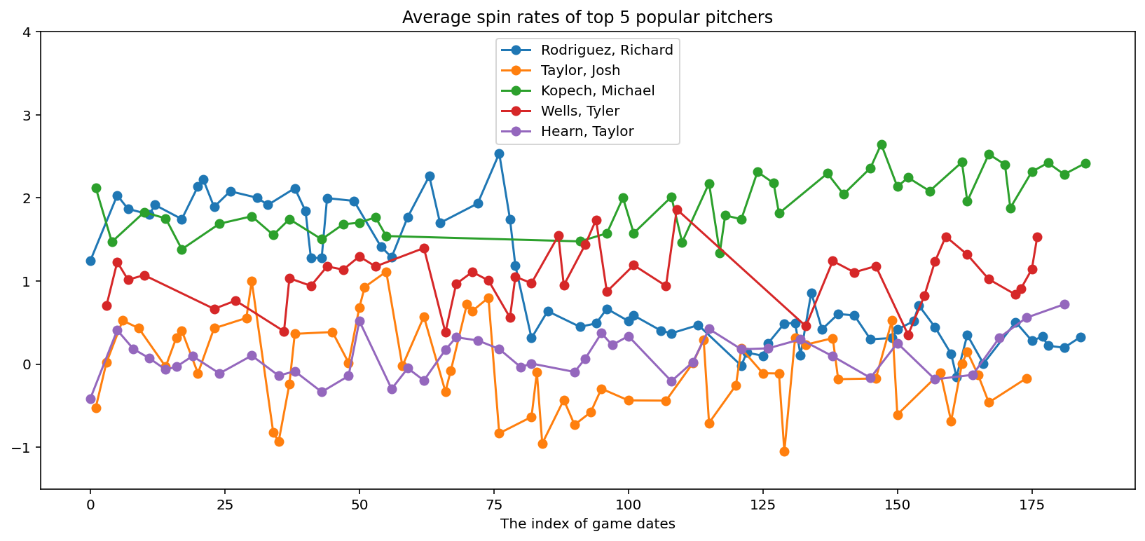
多输出高斯过程的优势在于它们能够同时学习和推断许多具有相同输入不确定性的输出。在这个例子中,我们从一个棒球数据集中对几位投手在不同比赛中的平均转速进行建模。
import arviz as az
import matplotlib.pyplot as plt
import numpy as np
import pandas as pd
import pymc as pm
import pytensor.tensor as pt

from pymc.gp.util import plot_gp_dist
%config InlineBackend.figure_format = 'retina'
RANDOM_SEED = 8927
rng = np.random.default_rng(RANDOM_SEED)
准备数据#
棒球数据集包含了几位投手在不同比赛日期的平均旋转率。
# get data
try:
    df = pd.read_csv("../data/fastball_spin_rates.csv")
except FileNotFoundError:
    df = pd.read_csv(pm.get_data("fastball_spin_rates.csv"))

print(df.shape)
df.head()
(4845, 4)
| pitcher_name | game_date | avg_spin_rate | n_pitches | |
|---|---|---|---|---|
| 0 | Wainwright, Adam | 2021-04-03 | 2127.415000 | 12 |
| 1 | Wainwright, Adam | 2021-04-08 | 2179.723000 | 11 |
| 2 | Wainwright, Adam | 2021-04-14 | 2297.968571 | 7 |
| 3 | Wainwright, Adam | 2021-04-20 | 2159.150000 | 13 |
| 4 | Wainwright, Adam | 2021-04-26 | 2314.515455 | 11 |
print(
    f"There are {df['pitcher_name'].nunique()} pitchers, in {df['game_date'].nunique()} game dates"
)
There are 262 pitchers, in 182 game dates
# Standardise average spin rate
df["avg_spin_rate"] = (df["avg_spin_rate"] - df["avg_spin_rate"].mean()) / df["avg_spin_rate"].std()
df["avg_spin_rate"].describe()
count    4.838000e+03
mean     1.821151e-16
std      1.000000e+00
min     -3.646438e+00
25%     -6.803556e-01
50%      4.736011e-03
75%      6.837128e-01
max      3.752720e+00
Name: avg_spin_rate, dtype: float64
前N名受欢迎的投手#
# Get top N popular pitchers by who attended most games
n_outputs = 5  # Top 5 popular pitchers
top_pitchers = df.groupby("pitcher_name")["game_date"].count().nlargest(n_outputs).reset_index()
top_pitchers = top_pitchers.reset_index().rename(columns={"index": "output_idx"})
top_pitchers
| output_idx | pitcher_name | game_date | |
|---|---|---|---|
| 0 | 0 | Rodriguez, Richard | 64 |
| 1 | 1 | Taylor, Josh | 59 |
| 2 | 2 | Kopech, Michael | 43 |
| 3 | 3 | Wells, Tyler | 43 |
| 4 | 4 | Hearn, Taylor | 42 |
# Filter the data with only top N pitchers
adf = df.loc[df["pitcher_name"].isin(top_pitchers["pitcher_name"])].copy()
print(adf.shape)
adf.head()
(251, 4)
| pitcher_name | game_date | avg_spin_rate | n_pitches | |
|---|---|---|---|---|
| 1631 | Rodriguez, Richard | 2021-04-01 | 1.245044 | 12 |
| 1632 | Rodriguez, Richard | 2021-04-06 | 2.032285 | 3 |
| 1633 | Rodriguez, Richard | 2021-04-08 | 1.868068 | 10 |
| 1634 | Rodriguez, Richard | 2021-04-12 | 1.801864 | 14 |
| 1635 | Rodriguez, Richard | 2021-04-13 | 1.916592 | 9 |
adf["avg_spin_rate"].describe()
count    251.000000
mean       0.774065
std        0.867510
min       -1.050933
25%        0.102922
50%        0.559293
75%        1.517114
max        2.647740
Name: avg_spin_rate, dtype: float64
创建一个游戏日期索引#
# There are 142 game dates from 01 Apr 2021 to 03 Oct 2021.
adf.loc[:, "game_date"] = pd.to_datetime(adf.loc[:, "game_date"])
game_dates = adf.loc[:, "game_date"]
game_dates.min(), game_dates.max(), game_dates.nunique(), (game_dates.max() - game_dates.min())
(Timestamp('2021-04-01 00:00:00'),
 Timestamp('2021-10-03 00:00:00'),
 142,
 Timedelta('185 days 00:00:00'))
# Create a game date index
dates_idx = pd.DataFrame(
    {"game_date": pd.date_range(game_dates.min(), game_dates.max())}
).reset_index()
dates_idx = dates_idx.rename(columns={"index": "x"})
dates_idx.head()
| x | game_date | |
|---|---|---|
| 0 | 0 | 2021-04-01 |
| 1 | 1 | 2021-04-02 |
| 2 | 2 | 2021-04-03 |
| 3 | 3 | 2021-04-04 |
| 4 | 4 | 2021-04-05 |
创建训练数据#
adf = adf.merge(dates_idx, how="left", on="game_date")
adf = adf.merge(top_pitchers[["pitcher_name", "output_idx"]], how="left", on="pitcher_name")
adf.head()
| pitcher_name | game_date | avg_spin_rate | n_pitches | x | output_idx | |
|---|---|---|---|---|---|---|
| 0 | Rodriguez, Richard | 2021-04-01 | 1.245044 | 12 | 0 | 0 |
| 1 | Rodriguez, Richard | 2021-04-06 | 2.032285 | 3 | 5 | 0 |
| 2 | Rodriguez, Richard | 2021-04-08 | 1.868068 | 10 | 7 | 0 |
| 3 | Rodriguez, Richard | 2021-04-12 | 1.801864 | 14 | 11 | 0 |
| 4 | Rodriguez, Richard | 2021-04-13 | 1.916592 | 9 | 12 | 0 |
adf = adf.sort_values(["output_idx", "x"])
X = adf[
    ["x", "output_idx"]
].values  # Input data includes the index of game dates, and the index of pitchers
Y = adf["avg_spin_rate"].values  # Output data includes the average spin rate of pitchers
X.shape, Y.shape
((251, 2), (251,))
可视化训练数据#
# Plot average spin rates of top pitchers
fig, ax = plt.subplots(1, 1, figsize=(14, 6))
legends = []
for pitcher in top_pitchers["pitcher_name"]:
    cond = adf["pitcher_name"] == pitcher
    ax.plot(adf.loc[cond, "x"], adf.loc[cond, "avg_spin_rate"], "-o")
    legends.append(pitcher)
plt.title("Average spin rates of top 5 popular pitchers")
plt.xlabel("The index of game dates")
plt.ylim([-1.5, 4.0])
plt.legend(legends, loc="upper center");
固有共区域化模型 (ICM)#
固有协同区域化模型(ICM)是线性协同区域化模型(LCM)的一个特例,具有一个输入核函数,例如:
其中 \(B(o,o')\) 是输出核,而 \(K_{ExpQuad}(x,x')\) 是输入核。
def get_icm(input_dim, kernel, W=None, kappa=None, B=None, active_dims=None):
    """
    This function generates an ICM kernel from an input kernel and a Coregion kernel.
    """
    coreg = pm.gp.cov.Coregion(input_dim=input_dim, W=W, kappa=kappa, B=B, active_dims=active_dims)
    icm_cov = kernel * coreg  # Use Hadamard Product for separate inputs
    return icm_cov
with pm.Model() as model:
    # Priors
    ell = pm.Gamma("ell", alpha=2, beta=0.5)
    eta = pm.Gamma("eta", alpha=3, beta=1)
    kernel = eta**2 * pm.gp.cov.ExpQuad(input_dim=2, ls=ell, active_dims=[0])
    sigma = pm.HalfNormal("sigma", sigma=3)

    # Get the ICM kernel
    W = pm.Normal("W", mu=0, sigma=3, shape=(n_outputs, 2), initval=np.random.randn(n_outputs, 2))
    kappa = pm.Gamma("kappa", alpha=1.5, beta=1, shape=n_outputs)
    B = pm.Deterministic("B", pt.dot(W, W.T) + pt.diag(kappa))
    cov_icm = get_icm(input_dim=2, kernel=kernel, B=B, active_dims=[1])

    # Define a Multi-output GP
    mogp = pm.gp.Marginal(cov_func=cov_icm)
    y_ = mogp.marginal_likelihood("f", X, Y, sigma=sigma)
pm.model_to_graphviz(model)

%%time
with model:
    gp_trace = pm.sample(2000, chains=1)
Auto-assigning NUTS sampler...
Initializing NUTS using jitter+adapt_diag...
Sequential sampling (1 chains in 1 job)
NUTS: [ell, eta, sigma, W, kappa]
Sampling 1 chain for 1_000 tune and 2_000 draw iterations (1_000 + 2_000 draws total) took 1278 seconds.
CPU times: user 46min 50s, sys: 2h 2min 57s, total: 2h 49min 47s
Wall time: 21min 25s
预测#
# Prepare test data
M = 200  # number of data points
x_new = np.linspace(0, 200, M)[
    :, None
]  # Select 200 days (185 previous days, and add 15 days into the future).
X_new = np.vstack([x_new for idx in range(n_outputs)])
output_idx = np.vstack([np.repeat(idx, M)[:, None] for idx in range(n_outputs)])
X_new = np.hstack([X_new, output_idx])
%%time
with model:
    preds = mogp.conditional("preds", X_new)
    gp_samples = pm.sample_posterior_predictive(gp_trace, var_names=["preds"], random_seed=42)
Sampling: [preds]
CPU times: user 46min 13s, sys: 39min 48s, total: 1h 26min 2s
Wall time: 10min 50s
f_pred = gp_samples.posterior_predictive["preds"].sel(chain=0)


def plot_predictive_posteriors(f_pred, top_pitchers, M, X_new):
    fig, axes = plt.subplots(n_outputs, 1, figsize=(12, 15))

    for idx, pitcher in enumerate(top_pitchers["pitcher_name"]):
        # Prediction
        plot_gp_dist(
            axes[idx],
            f_pred[:, M * idx : M * (idx + 1)],
            X_new[M * idx : M * (idx + 1), 0],
            palette="Blues",
            fill_alpha=0.1,
            samples_alpha=0.1,
        )
        # Training data points
        cond = adf["pitcher_name"] == pitcher
        axes[idx].scatter(adf.loc[cond, "x"], adf.loc[cond, "avg_spin_rate"], color="r")
        axes[idx].set_title(pitcher)
    plt.tight_layout()


plot_predictive_posteriors(f_pred, top_pitchers, M, X_new)
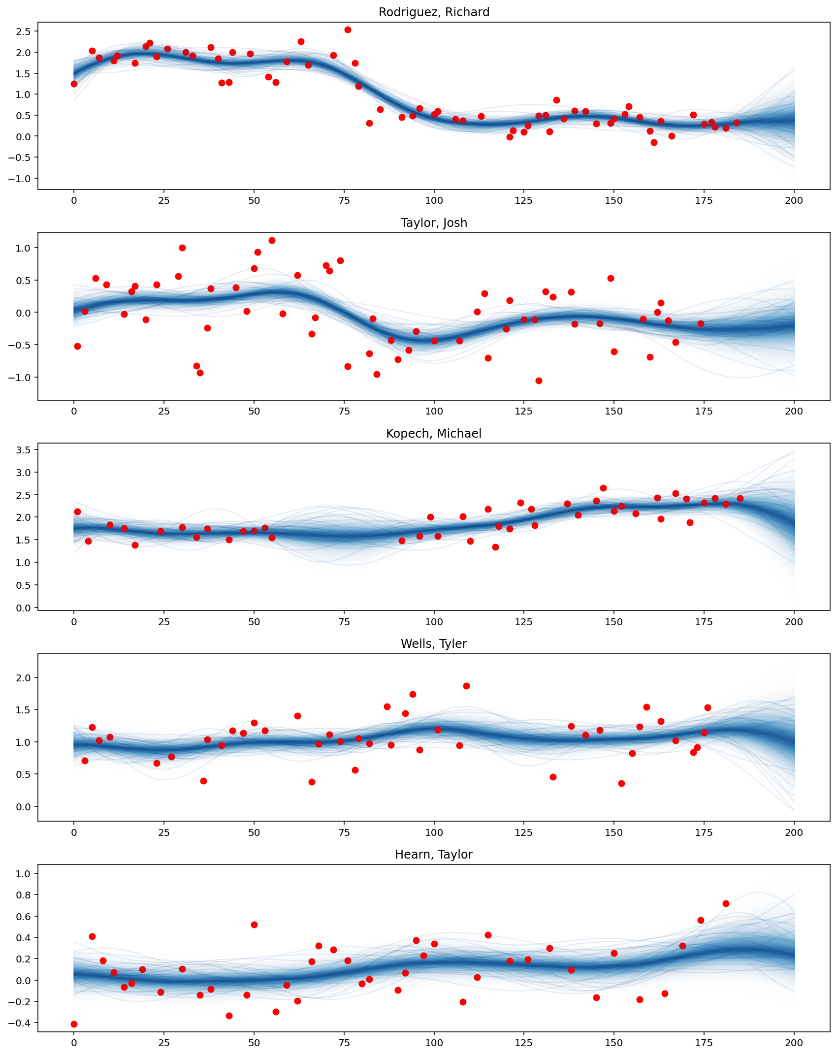
可以看出,Rodriguez Richard 的平均旋转速率从第75场比赛日期开始显著下降。此外,Kopech Michael 在中断几周后表现有所提升,而 Hearn Taylor 最近表现更好。
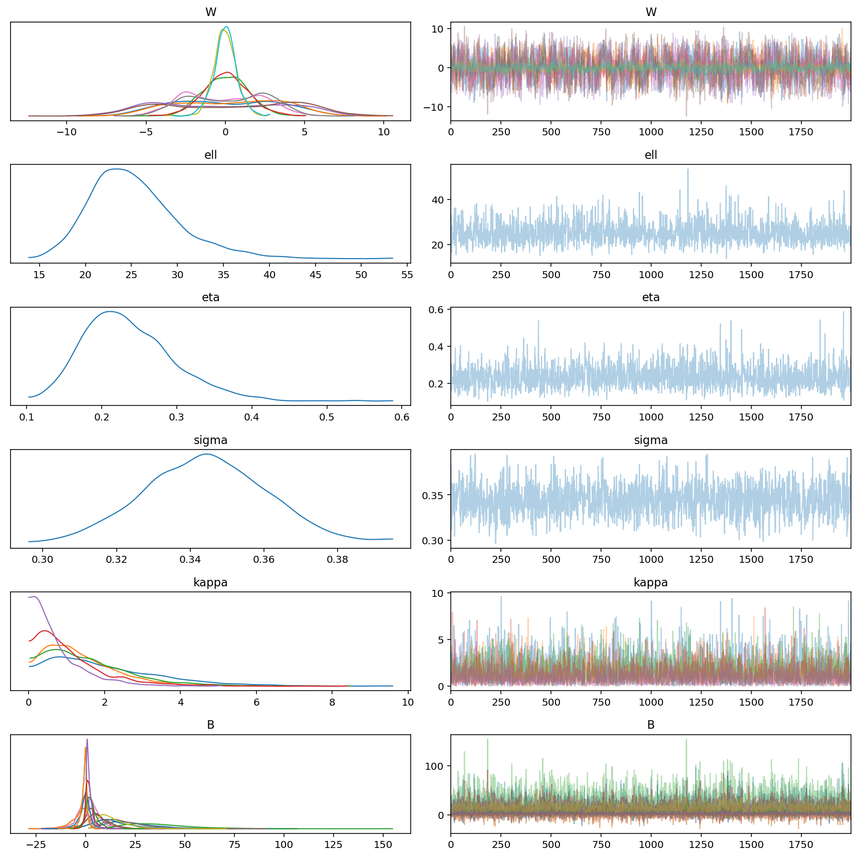
az.plot_trace(gp_trace)
plt.tight_layout()
线性协同区域化模型 (LCM)#
LCM 是 ICM 的推广,具有两个或更多输入核,因此 LCM 核基本上是几个 ICM 核的总和。LMC 允许从具有不同协方差(核)的 GP 中进行几个独立样本。
在这个例子中,除了一个ExpQuad核函数外,我们还为输入数据添加了一个Matern32核函数。
def get_lcm(input_dim, active_dims, num_outputs, kernels, W=None, B=None, name="ICM"):
    """
    This function generates a LCM kernel from a list of input `kernels` and a Coregion kernel.
    """
    if B is None:
        kappa = pm.Gamma(f"{name}_kappa", alpha=5, beta=1, shape=num_outputs)
        if W is None:
            W = pm.Normal(
                f"{name}_W",
                mu=0,
                sigma=5,
                shape=(num_outputs, 1),
                initval=np.random.randn(num_outputs, 1),
            )
    else:
        kappa = None

    cov_func = 0
    for idx, kernel in enumerate(kernels):
        icm = get_icm(input_dim, kernel, W, kappa, B, active_dims)
        cov_func += icm
    return cov_func
with pm.Model() as model:
    # Priors
    ell = pm.Gamma("ell", alpha=2, beta=0.5, shape=2)
    eta = pm.Gamma("eta", alpha=3, beta=1, shape=2)
    kernels = [pm.gp.cov.ExpQuad, pm.gp.cov.Matern32]
    sigma = pm.HalfNormal("sigma", sigma=3)

    # Define a list of covariance functions
    cov_list = [
        eta[idx] ** 2 * kernel(input_dim=2, ls=ell[idx], active_dims=[0])
        for idx, kernel in enumerate(kernels)
    ]

    # Get the LCM kernel
    cov_lcm = get_lcm(input_dim=2, active_dims=[1], num_outputs=n_outputs, kernels=cov_list)

    # Define a Multi-output GP
    mogp = pm.gp.Marginal(cov_func=cov_lcm)
    y_ = mogp.marginal_likelihood("f", X, Y, sigma=sigma)
pm.model_to_graphviz(model)

%%time
with model:
    gp_trace = pm.sample(2000, chains=1)
Auto-assigning NUTS sampler...
Initializing NUTS using jitter+adapt_diag...
Sequential sampling (1 chains in 1 job)
NUTS: [ell, eta, sigma, ICM_kappa, ICM_W]
Sampling 1 chain for 1_000 tune and 2_000 draw iterations (1_000 + 2_000 draws total) took 1109 seconds.
There were 2 divergences after tuning. Increase `target_accept` or reparameterize.
CPU times: user 40min 37s, sys: 1h 47min 9s, total: 2h 27min 46s
Wall time: 18min 39s
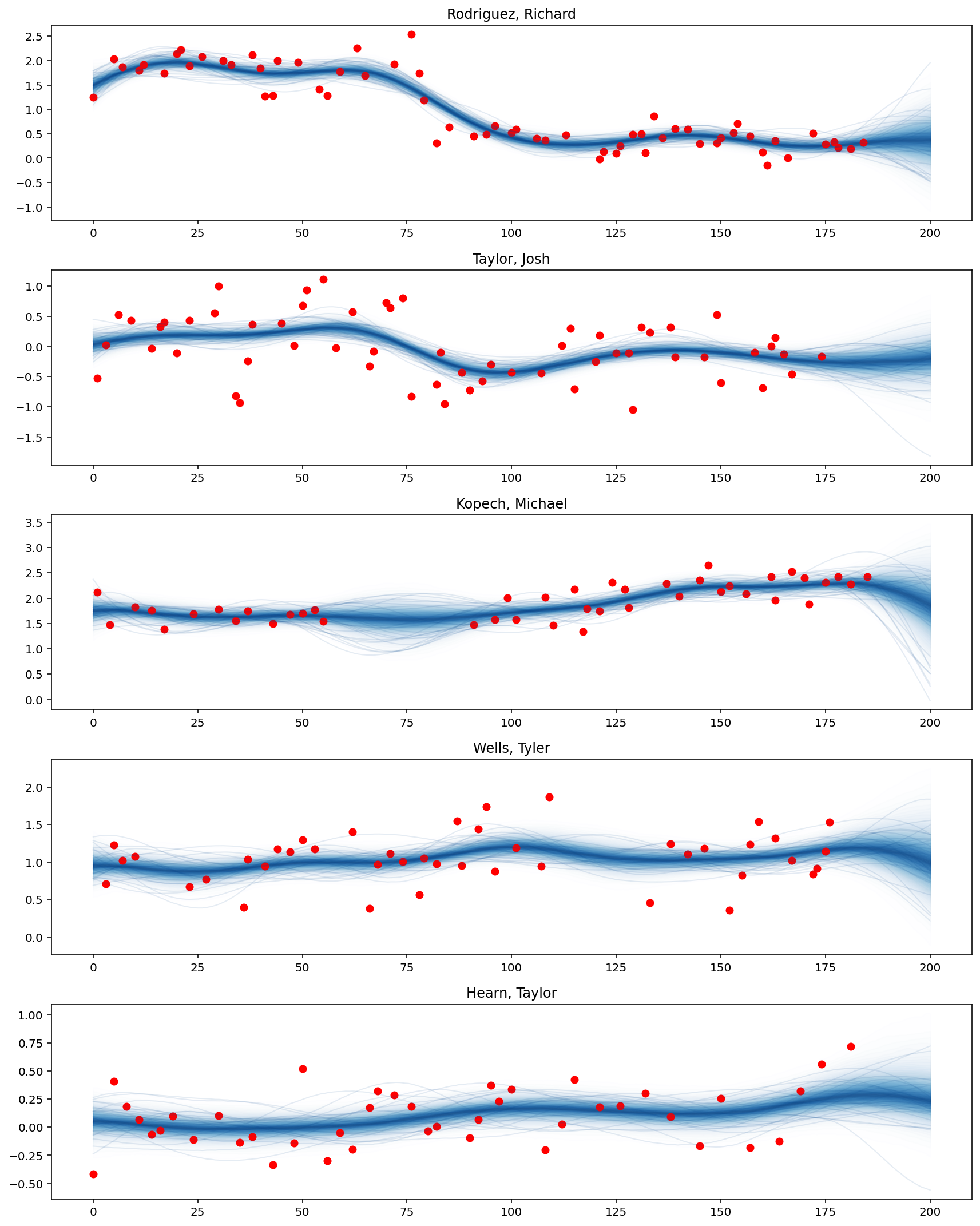
预测#
%%time
with model:
    preds = mogp.conditional("preds", X_new)
    gp_samples = pm.sample_posterior_predictive(gp_trace, var_names=["preds"], random_seed=42)
Sampling: [preds]
CPU times: user 51min 44s, sys: 50min 14s, total: 1h 41min 59s
Wall time: 12min 53s
plot_predictive_posteriors(f_pred, top_pitchers, M, X_new)
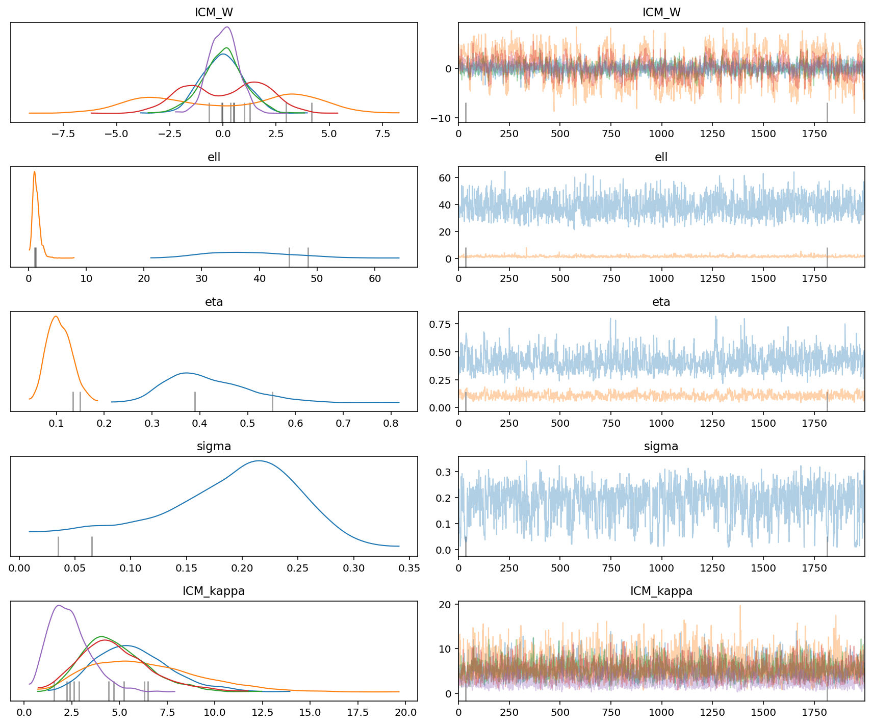
az.plot_trace(gp_trace)
plt.tight_layout()
致谢#
这项工作得到了2022年Google Summer of Codes和NUMFOCUS的支持。
参考资料#
Edwin V Bonilla, Kian Chai, 和 Christopher Williams. 多任务高斯过程预测. 神经信息处理系统进展, 2007. URL: https://papers.nips.cc/paper/2007/hash/66368270ffd51418ec58bd793f2d9b1b-Abstract.html.
水印#
%load_ext watermark
%watermark -n -u -v -iv -w -p pytensor,aeppl,xarray
The watermark extension is already loaded. To reload it, use:
  %reload_ext watermark
Last updated: Sat Nov 12 2022

Python implementation: CPython
Python version       : 3.9.12
IPython version      : 8.3.0

pytensor: 2.8.6
aeppl : 0.0.36
xarray: 2022.3.0

pymc      : 4.2.1
arviz     : 0.13.0
pandas    : 1.4.2
pytensor    : 2.8.6
numpy     : 1.22.4
matplotlib: 3.5.2

Watermark: 2.3.0
许可证通知#
本示例库中的所有笔记本均在MIT许可证下提供,该许可证允许修改和重新分发,前提是保留版权和许可证声明。
引用 PyMC 示例#
要引用此笔记本,请使用Zenodo为pymc-examples仓库提供的DOI。
重要
许多笔记本是从其他来源改编的:博客、书籍……在这种情况下,您应该引用原始来源。
还要记得引用代码中使用的相关库。
这是一个BibTeX的引用模板:
@incollection{citekey,
  author    = "<notebook authors, see above>",
  title     = "<notebook title>",
  editor    = "PyMC Team",
  booktitle = "PyMC examples",
  doi       = "10.5281/zenodo.5654871"
}
渲染后可能看起来像: