


有序分类结果的回归模型#
import arviz as az
import matplotlib.pyplot as plt
import numpy as np
import pandas as pd
import pymc as pm
import pytensor.tensor as pt
import statsmodels.api as sm

from scipy.stats import bernoulli
from statsmodels.miscmodels.ordinal_model import OrderedModel
%config InlineBackend.figure_format = 'retina'  # high resolution figures
az.style.use("arviz-darkgrid")
rng = np.random.default_rng(42)
序数尺度和调查数据#
与统计学的许多领域一样,调查数据的语言也带有词汇过载的特点。在讨论调查设计时,您经常会听到关于基于设计和基于模型的方法之间的对比,这些方法涉及(i)抽样策略和(ii)对相关数据的统计推断。我们不会深入探讨不同的抽样策略的细节,例如:简单随机抽样、整群随机抽样或使用人口加权方案的分层随机抽样。关于这些策略的文献非常丰富,但在本笔记本中,我们将讨论何时以及为什么将模型驱动的统计推断应用于Likert量表的调查响应数据和其他类型的有序分类数据是有用的。
有序类别:已知分布#
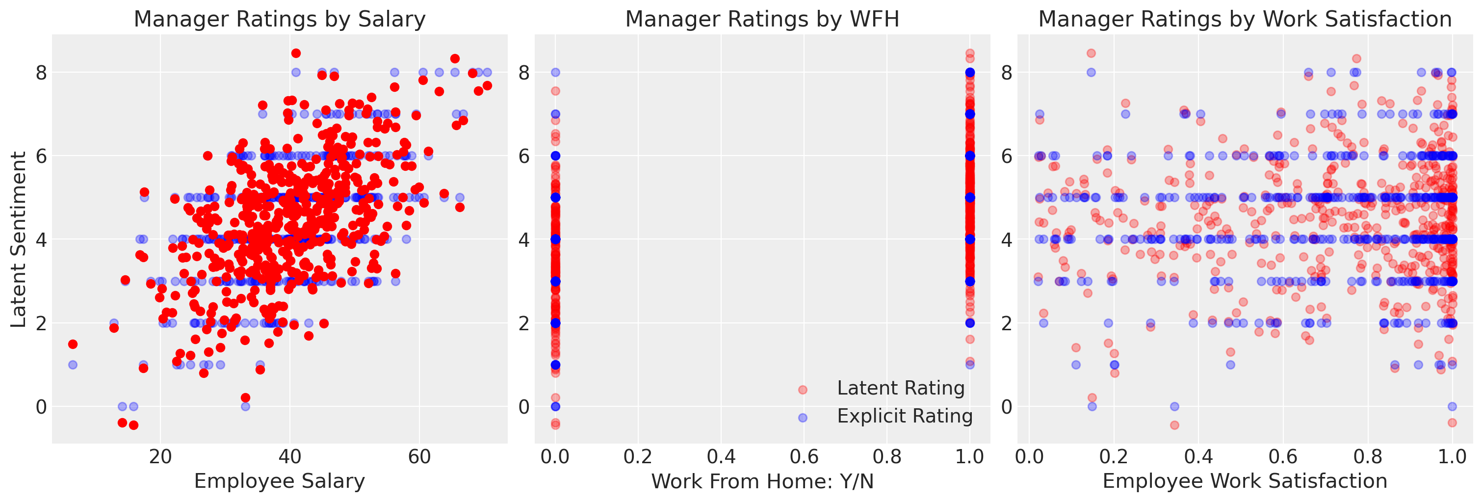
我们将从生成一些假数据开始。想象一个员工/经理关系,其中年度流程的一部分涉及进行360度评估。经理会得到一个评分(1 - 10),由他们的团队和人力资源部门收集这些评分。人力资源经理想知道哪些因素影响经理的评分,以及如何将获得4分的经理提升到5分,或将获得7分的经理提升到8分。他们有一个理论,即评分很大程度上是工资的函数。
序数回归是一种统计技术,旨在建模这些类型的关系,并且可以与基于设计的方法形成对比,后者的重点是提取简单的统计摘要,例如在调查设计背景下,在关于这些派生摘要的误差容限有强保证的情况下,提取比例、计数或比率。
def make_data():
    np.random.seed(100)
    salary = np.random.normal(40, 10, 500)
    work_sat = np.random.beta(1, 0.4, 500)
    work_from_home = bernoulli.rvs(0.7, size=500)
    work_from_home_calc = np.where(work_from_home, 1.4 * work_from_home, work_from_home)
    latent_rating = (
        0.08423 * salary + 0.2 * work_sat + work_from_home_calc + np.random.normal(0, 1, 500)
    )
    explicit_rating = np.round(latent_rating, 0)
    df = pd.DataFrame(
        {
            "salary": salary,
            "work_sat": work_sat,
            "work_from_home": work_from_home,
            "latent_rating": latent_rating,
            "explicit_rating": explicit_rating,
        }
    )
    return df


try:
    df = pd.read_csv("../data/fake_employee_manger_rating.csv")
    df = df[["salary", "work_sat", "work_from_home", "latent_rating", "explicit_rating"]]
except FileNotFoundError:
    df = make_data()

K = len(df["explicit_rating"].unique())
df.head()
| salary | work_sat | work_from_home | latent_rating | explicit_rating | |
|---|---|---|---|---|---|
| 0 | 41.172474 | 0.632002 | 1 | 5.328188 | 5.0 |
| 1 | 40.984524 | 0.904452 | 0 | 3.198263 | 3.0 |
| 2 | 36.469472 | 0.911330 | 1 | 4.108042 | 4.0 |
| 3 | 6.453822 | 0.919106 | 0 | 1.496440 | 1.0 |
| 4 | 33.795497 | 0.894581 | 0 | 3.200672 | 3.0 |
我们已经以一种方式指定了数据,使得存在一个潜在的情感,它是连续的尺度,被粗略地离散化为表示有序的评级尺度。我们已经以一种方式指定了数据,使得薪水驱动了经理评级相当线性的增加。
fig, axs = plt.subplots(1, 3, figsize=(15, 5))
axs = axs.flatten()
ax = axs[0]
ax.scatter(df["salary"], df["explicit_rating"], label="Explicit Rating", color="blue", alpha=0.3)
axs[1].scatter(
    df["work_from_home"], df["latent_rating"], label="Latent Rating", color="red", alpha=0.3
)
axs[1].scatter(
    df["work_from_home"], df["explicit_rating"], label="Explicit Rating", c="blue", alpha=0.3
)
axs[2].scatter(df["work_sat"], df["latent_rating"], label="Latent Rating", color="red", alpha=0.3)
axs[2].scatter(
    df["work_sat"], df["explicit_rating"], label="Explicit Rating", color="blue", alpha=0.3
)
ax.scatter(df["salary"], df["latent_rating"], label="Latent Sentiment", color="red")
ax.set_title("Manager Ratings by Salary")
axs[1].set_title("Manager Ratings by WFH")
axs[2].set_title("Manager Ratings by Work Satisfaction")
ax.set_ylabel("Latent Sentiment")
ax.set_xlabel("Employee Salary")
axs[1].set_xlabel("Work From Home: Y/N")
axs[2].set_xlabel("Employee Work Satisfaction")
axs[1].legend();
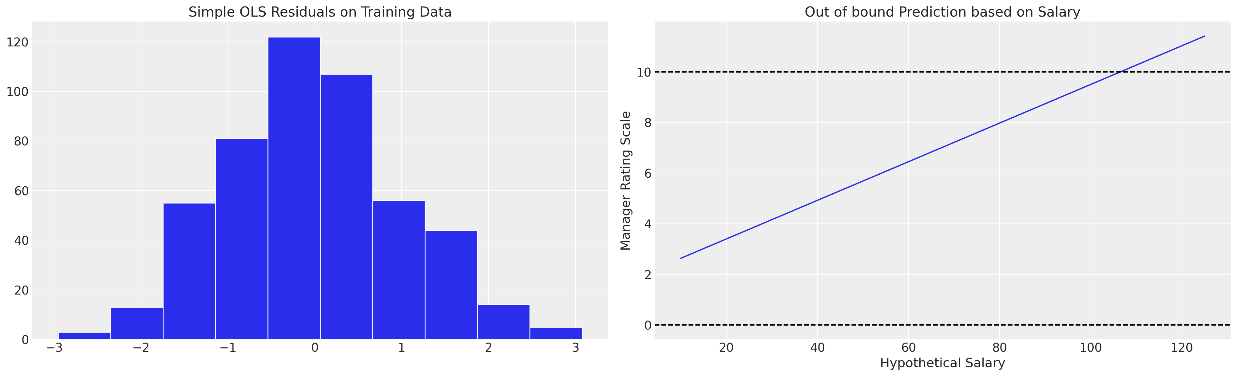
然而,我们可以看到,如果我们用简单的OLS拟合来拟合这个模型,它暗示了超出分类尺度的值,这可能会激励过于热心的HR经理提供虚假的加薪。OLS近似法的局限性在于它无法解释结果变量的正确性质。
exog = sm.add_constant(df[["salary", "work_from_home", "work_sat"]])
mod = sm.OLS(df["explicit_rating"], exog)
results = mod.fit()
results.summary()

results.predict([1, 200, 1, 0.6])
fig, axs = plt.subplots(1, 2, figsize=(20, 6))
axs = axs.flatten()
ax = axs[1]
salaries = np.linspace(10, 125, 20)
predictions = [results.predict([1, i, 1, 0.6])[0] for i in salaries]
ax.plot(salaries, predictions, label="Implied Linear function of Salaries on Outcome")
ax.set_title("Out of bound Prediction based on Salary")
ax.axhline(10, linestyle="--", color="black")
ax.set_xlabel("Hypothetical Salary")
ax.set_ylabel("Manager Rating Scale")
ax.axhline(0, linestyle="--", color="black")
axs[0].hist(results.resid, ec="white")
axs[0].set_title("Simple OLS Residuals on Training Data");
这表明了在基于设计和模型的调查数据推理方法之间存在对比的原因。建模方法通常隐藏或埋没假设,这使得模型不可行,而保守的方法倾向于在设计理念下进行推理,以避免模型错误指定的风险。
序数回归模型:概念#
在本笔记本中,我们将展示如何拟合回归模型以避免一类模型错误指定的问题。这些类型的模型可以被视为在潜在连续尺度上具有多个阈值的逻辑回归模型的应用。其思想是存在一个潜在的度量标准,可以通过度量的极端程度进行划分,但我们只观察到个体所在的尺度分区指标。这是一个非常自然的视角,例如想象在粗略的政治分类中隐藏的复杂性:自由派、温和派和保守派。你可能对许多政治问题有一系列观点,但它们在政治计算中都被简化为有限的一组(通常是糟糕的)选择。在过去的10个政治选择中,哪一个将你从自由派推向了温和派?
这个想法是将结果变量(我们的分类)判断视为源自一个潜在的连续测量。我们看到的这些结果只是在那个连续测量达到某个阈值时才会出现。序数回归的主要推断任务是推导出潜在连续空间中这些阈值的估计值。
在上面的数据集中,我们明确指定了关系,在接下来的步骤中,我们将估计各种有序回归模型。
拟合多种模型规格#
序数回归模型的模型规范通常使用logit变换和隐含的累积概率。对于具有概率\(\pi_1, .... \pi_n\)的\(c\)个结果类别,累积对数比率定义为:
这在回归上下文中被使用,我们以线性方式指定决定我们潜在结果的因素:
这意味着:
并且属于某个特定类别 \(j\) 的概率由以下单元格定义的概率决定:
以这种方式指定的序数回归的一个优点是,在潜在空间上的每个区间内,beta项系数的解释保持不变。模型参数的解释是典型的:\(x_{k}\) 的单位增加对应于 \(Y_{latent}\) 增加 \(\beta_{k}\)。类似的解释也适用于概率回归规范。然而,我们必须小心比较不同模型规范中不同变量的系数解释。上述系数解释在基于固定模型中变量的条件解释下是有意义的。添加或删除变量会改变条件化,这会由于非折叠现象而破坏模型的可比性。我们将在下面展示如何通过使用后验预测分布来更好地比较模型的预测含义。
贝叶斯特性#
虽然序数回归通常在频率主义范式中进行,但同样的技术可以在贝叶斯环境中应用,从而获得后验概率分布和后验预测模拟的所有好处。在PyMC中,我们至少有两种方法可以指定该模型的先验。第一种方法使用受限的Dirichlet分布来定义阈值的先验。第二种方法稍微宽松一些,允许指定任何具有适当数量切点的先验分布,并对从先验分布生成的样本应用排序变换。
我们将在本笔记本中展示这两种方法,但正如我们将看到的,Dirichlet的定义确保了使其更适合受限结果空间的特性。在每种方法中,我们都可以像在更标准的回归模型中一样包含协变量。
PyMC 提供了 OrderedLogistic 和 OrderedProbit 分布。
def constrainedUniform(N, min=0, max=1):
    return pm.Deterministic(
        "cutpoints",
        pt.concatenate(
            [
                np.ones(1) * min,
                pt.extra_ops.cumsum(pm.Dirichlet("cuts_unknown", a=np.ones(N - 2))) * (max - min)
                + min,
            ]
        ),
    )
上述函数(由Ben Vincent博士和Adrian Seyboldt提出)看起来有些令人畏惧,但它只是一个方便的函数,用于在我们的\(Y_{latent}\)中指定一个关于切点的先验。Dirichlet分布的特殊之处在于,从该分布中抽取的样本必须总和为一。上述函数确保了从先验分布中抽取的每个样本都是我们有序分类中最大类别大于最小值的累积份额。
def make_model(priors, model_spec=1, constrained_uniform=False, logit=True):
    with pm.Model() as model:
        if constrained_uniform:
            cutpoints = constrainedUniform(K, 0, K)
        else:
            sigma = pm.Exponential("sigma", priors["sigma"])
            cutpoints = pm.Normal(
                "cutpoints",
                mu=priors["mu"],
                sigma=sigma,
                transform=pm.distributions.transforms.univariate_ordered,
            )

        if model_spec == 1:
            beta = pm.Normal("beta", priors["beta"][0], priors["beta"][1], size=1)
            mu = pm.Deterministic("mu", beta[0] * df.salary)
        elif model_spec == 2:
            beta = pm.Normal("beta", priors["beta"][0], priors["beta"][1], size=2)
            mu = pm.Deterministic("mu", beta[0] * df.salary + beta[1] * df.work_sat)
        elif model_spec == 3:
            beta = pm.Normal("beta", priors["beta"][0], priors["beta"][1], size=3)
            mu = pm.Deterministic(
                "mu", beta[0] * df.salary + beta[1] * df.work_sat + beta[2] * df.work_from_home
            )
        if logit:
            y_ = pm.OrderedLogistic("y", cutpoints=cutpoints, eta=mu, observed=df.explicit_rating)
        else:
            y_ = pm.OrderedProbit("y", cutpoints=cutpoints, eta=mu, observed=df.explicit_rating)
        idata = pm.sample(nuts_sampler="numpyro", idata_kwargs={"log_likelihood": True})
        idata.extend(pm.sample_posterior_predictive(idata))
    return idata, model


priors = {"sigma": 1, "beta": [0, 1], "mu": np.linspace(0, K, K - 1)}
idata1, model1 = make_model(priors, model_spec=1)
idata2, model2 = make_model(priors, model_spec=2)
idata3, model3 = make_model(priors, model_spec=3)
idata4, model4 = make_model(priors, model_spec=3, constrained_uniform=True)
idata5, model5 = make_model(priors, model_spec=3, constrained_uniform=True)
Show code cell output
/Users/nathanielforde/mambaforge/envs/pymc_examples_new/lib/python3.9/site-packages/pymc/sampling/mcmc.py:243: UserWarning: Use of external NUTS sampler is still experimental
  warnings.warn("Use of external NUTS sampler is still experimental", UserWarning)
Compiling...
Compilation time =  0:00:01.829062
Sampling...
Sampling time =  0:00:05.483080
Transforming variables...
Transformation time =  0:00:00.442042
Computing Log Likelihood...
/Users/nathanielforde/mambaforge/envs/pymc_examples_new/lib/python3.9/site-packages/pymc/sampling/mcmc.py:243: UserWarning: Use of external NUTS sampler is still experimental
  warnings.warn("Use of external NUTS sampler is still experimental", UserWarning)
Compiling...
Compilation time =  0:00:02.785476
Sampling...
Sampling time =  0:00:05.161887
Transforming variables...
Transformation time =  0:00:00.215416
Computing Log Likelihood...
/Users/nathanielforde/mambaforge/envs/pymc_examples_new/lib/python3.9/site-packages/pymc/sampling/mcmc.py:243: UserWarning: Use of external NUTS sampler is still experimental
  warnings.warn("Use of external NUTS sampler is still experimental", UserWarning)
Compiling...
Compilation time =  0:00:01.304173
Sampling...
Sampling time =  0:00:06.041616
Transforming variables...
Transformation time =  0:00:00.174980
Computing Log Likelihood...
/Users/nathanielforde/mambaforge/envs/pymc_examples_new/lib/python3.9/site-packages/pymc/sampling/mcmc.py:243: UserWarning: Use of external NUTS sampler is still experimental
  warnings.warn("Use of external NUTS sampler is still experimental", UserWarning)
Compiling...
Compilation time =  0:00:02.029193
Sampling...
Sampling time =  0:00:04.205211
Transforming variables...
Transformation time =  0:00:00.332793
Computing Log Likelihood...
/Users/nathanielforde/mambaforge/envs/pymc_examples_new/lib/python3.9/site-packages/pymc/sampling/mcmc.py:243: UserWarning: Use of external NUTS sampler is still experimental
  warnings.warn("Use of external NUTS sampler is still experimental", UserWarning)
Compiling...
Compilation time =  0:00:01.665197
Sampling...
Sampling time =  0:00:04.125931
Transforming variables...
Transformation time =  0:00:00.174673
Computing Log Likelihood...
az.summary(idata3, var_names=["sigma", "cutpoints", "beta"])
| mean | sd | hdi_3% | hdi_97% | mcse_mean | mcse_sd | ess_bulk | ess_tail | r_hat | |
|---|---|---|---|---|---|---|---|---|---|
| sigma | 2.039 | 0.622 | 0.976 | 3.212 | 0.012 | 0.008 | 2782.0 | 2623.0 | 1.0 |
| cutpoints[0] | -1.639 | 0.793 | -3.173 | -0.239 | 0.015 | 0.011 | 2810.0 | 2564.0 | 1.0 |
| cutpoints[1] | 1.262 | 0.464 | 0.409 | 2.139 | 0.007 | 0.005 | 4086.0 | 3251.0 | 1.0 |
| cutpoints[2] | 3.389 | 0.441 | 2.598 | 4.249 | 0.008 | 0.005 | 3252.0 | 3280.0 | 1.0 |
| cutpoints[3] | 5.074 | 0.466 | 4.179 | 5.941 | 0.009 | 0.006 | 2850.0 | 2614.0 | 1.0 |
| cutpoints[4] | 6.886 | 0.508 | 5.964 | 7.875 | 0.010 | 0.007 | 2558.0 | 2924.0 | 1.0 |
| cutpoints[5] | 8.765 | 0.563 | 7.664 | 9.800 | 0.011 | 0.008 | 2440.0 | 3031.0 | 1.0 |
| cutpoints[6] | 10.338 | 0.614 | 9.183 | 11.505 | 0.012 | 0.009 | 2475.0 | 2949.0 | 1.0 |
| cutpoints[7] | 12.316 | 0.722 | 11.030 | 13.758 | 0.014 | 0.010 | 2633.0 | 3016.0 | 1.0 |
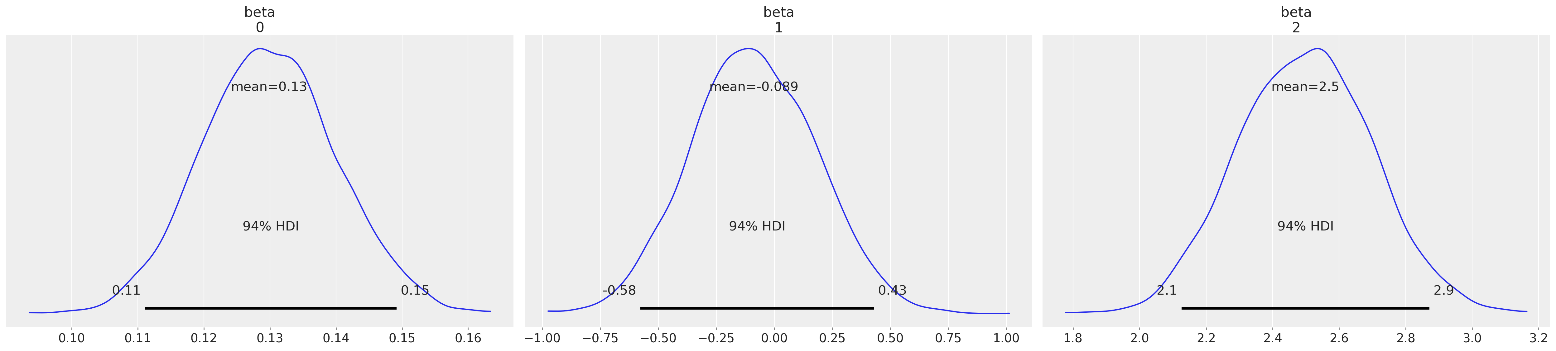
| beta[0] | 0.130 | 0.010 | 0.111 | 0.149 | 0.000 | 0.000 | 3069.0 | 3306.0 | 1.0 |
| beta[1] | -0.089 | 0.270 | -0.577 | 0.428 | 0.004 | 0.004 | 5076.0 | 2915.0 | 1.0 |
| beta[2] | 2.498 | 0.201 | 2.126 | 2.871 | 0.004 | 0.003 | 3161.0 | 2944.0 | 1.0 |
pm.model_to_graphviz(model3)

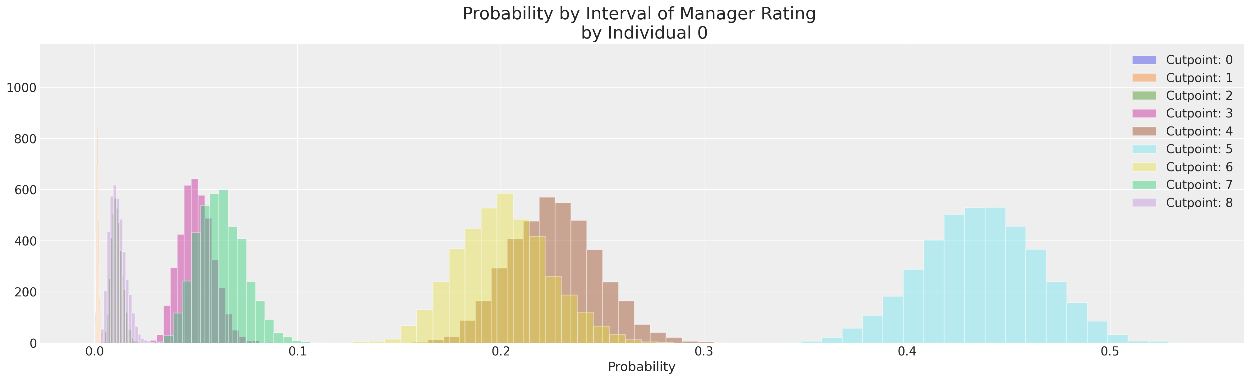
提取单个概率#
我们现在可以为每位经理的评分,查看与每个可用类别相关的概率。在我们后验分布的各个部分中,可以看到员工最有可能落在潜在连续测量的哪个部分。
implied_probs = az.extract(idata3, var_names=["y_probs"])
implied_probs.shape
(500, 9, 4000)
implied_probs[0].mean(axis=1)
<xarray.DataArray 'y_probs' (y_probs_dim_1: 9)>
array([1.11373333e-04, 1.47134815e-03, 1.08968413e-02, 5.03528852e-02,
       2.26303020e-01, 4.36314380e-01, 2.00984249e-01, 6.21568993e-02,
       1.14090037e-02])
Coordinates:
    y_probs_dim_0  int64 0
* y_probs_dim_1 (y_probs_dim_1) int64 0 1 2 3 4 5 6 7 8fig, ax = plt.subplots(figsize=(20, 6))
for i in range(K):
ax.hist(implied_probs[0, i, :], label=f"Cutpoint: {i}", ec="white", bins=20, alpha=0.4)
ax.set_xlabel("Probability")
ax.set_title("Probability by Interval of Manager Rating \n by Individual 0", fontsize=20)
ax.legend();
implied_class = az.extract(idata3, var_names=["y"], group="posterior_predictive")
implied_class.shape
(500, 4000)
from scipy.stats import mode
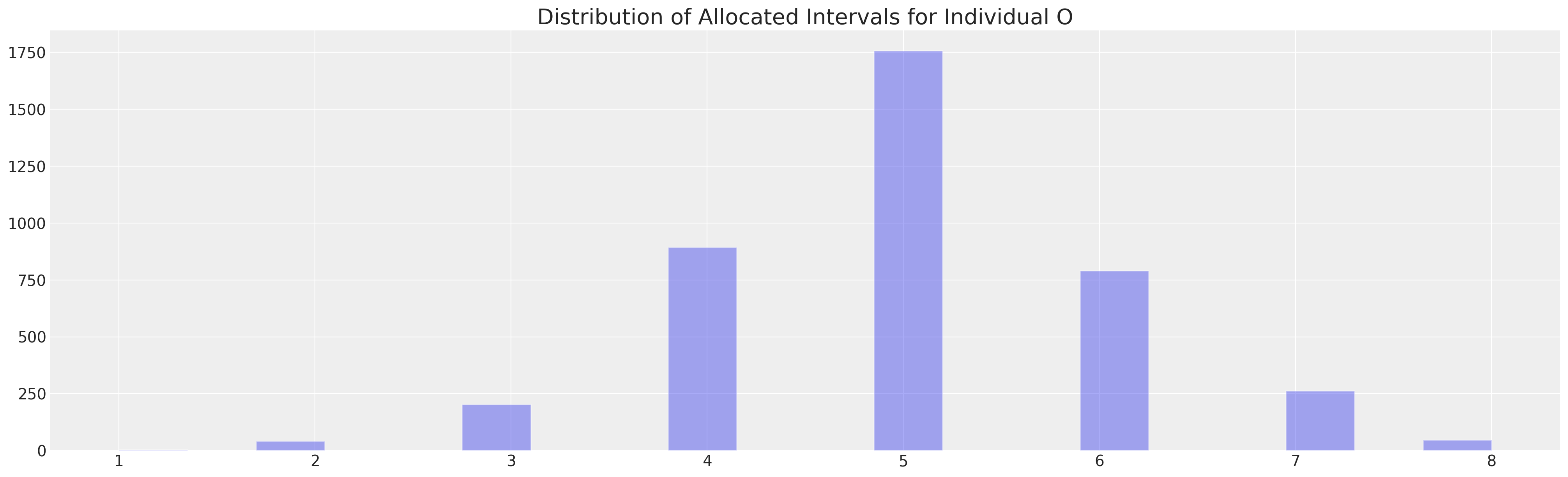
mode(implied_class[0])
/var/folders/__/ng_3_9pn1f11ftyml_qr69vh0000gn/T/ipykernel_63059/3774112.py:3: FutureWarning: Unlike other reduction functions (e.g. `skew`, `kurtosis`), the default behavior of `mode` typically preserves the axis it acts along. In SciPy 1.11.0, this behavior will change: the default value of `keepdims` will become False, the `axis` over which the statistic is taken will be eliminated, and the value None will no longer be accepted. Set `keepdims` to True or False to avoid this warning.
  mode(implied_class[0])
ModeResult(mode=array([5]), count=array([1758]))
fig, ax = plt.subplots(figsize=(20, 6))
ax.hist(implied_class[0], ec="white", bins=20, alpha=0.4)
ax.set_title("Distribution of Allocated Intervals for Individual O", fontsize=20);
比较模型:参数拟合和LOO#
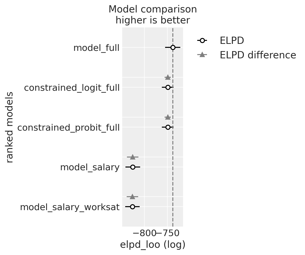
用于改善模型错误指定风险的一个工具是比较不同的候选模型以检查预测准确性。
compare = az.compare(
    {
        "model_salary": idata1,
        "model_salary_worksat": idata2,
        "model_full": idata3,
        "constrained_logit_full": idata4,
        "constrained_probit_full": idata5,
    }
)

az.plot_compare(compare)
compare
| rank | elpd_loo | p_loo | elpd_diff | weight | se | dse | warning | scale | |
|---|---|---|---|---|---|---|---|---|---|
| model_full | 0 | -738.115609 | 11.514954 | 0.000000 | 8.089471e-01 | 16.676300 | 0.000000 | False | log |
| constrained_logit_full | 1 | -748.997150 | 7.502048 | 10.881541 | 1.910529e-01 | 12.737133 | 6.778651 | False | log |
| constrained_probit_full | 2 | -749.078203 | 7.580680 | 10.962594 | 3.124925e-14 | 12.730696 | 6.776967 | False | log |
| model_salary | 3 | -825.636071 | 8.339788 | 87.520462 | 1.785498e-14 | 15.967569 | 12.472026 | False | log |
| model_salary_worksat | 4 | -826.443265 | 9.272995 | 88.327656 | 0.000000e+00 | 15.911693 | 12.464281 | False | log |
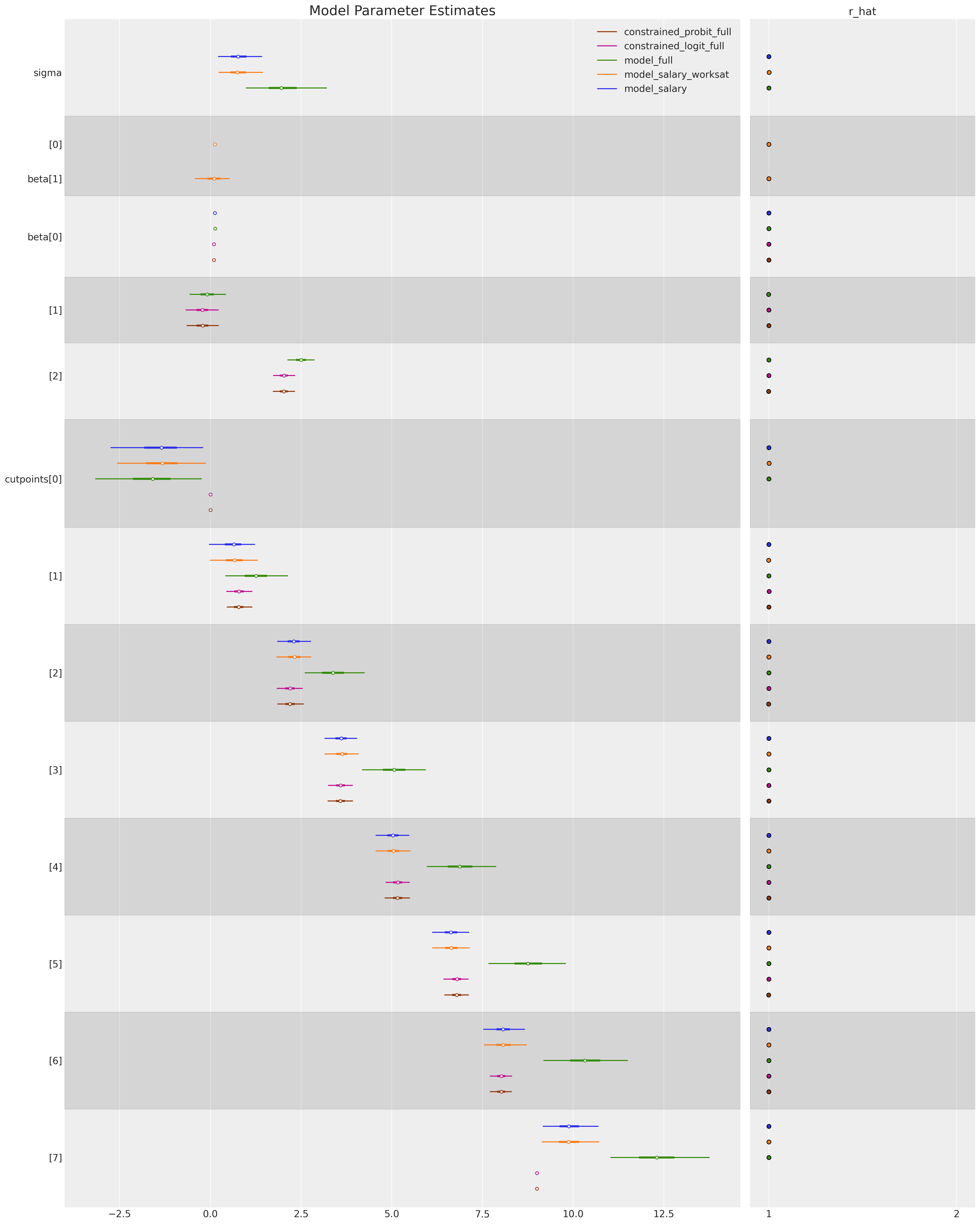
我们还可以比较控制每个回归模型的估计参数,以查看我们的模型拟合对替代参数化的稳健性。
ax = az.plot_forest(
    [idata1, idata2, idata3, idata4, idata5],
    var_names=["sigma", "beta", "cutpoints"],
    combined=True,
    ridgeplot_overlap=4,
    figsize=(20, 25),
    r_hat=True,
    ridgeplot_alpha=0.3,
    model_names=[
        "model_salary",
        "model_salary_worksat",
        "model_full",
        "constrained_logit_full",
        "constrained_probit_full",
    ],
)
ax[0].set_title("Model Parameter Estimates", fontsize=20);
/Users/nathanielforde/mambaforge/envs/pymc_examples_new/lib/python3.9/site-packages/arviz/stats/diagnostics.py:592: RuntimeWarning: invalid value encountered in double_scalars
  (between_chain_variance / within_chain_variance + num_samples - 1) / (num_samples)
az.summary(idata3, var_names=["cutpoints", "beta", "sigma"])
| mean | sd | hdi_3% | hdi_97% | mcse_mean | mcse_sd | ess_bulk | ess_tail | r_hat | |
|---|---|---|---|---|---|---|---|---|---|
| cutpoints[0] | -1.639 | 0.793 | -3.173 | -0.239 | 0.015 | 0.011 | 2810.0 | 2564.0 | 1.0 |
| cutpoints[1] | 1.262 | 0.464 | 0.409 | 2.139 | 0.007 | 0.005 | 4086.0 | 3251.0 | 1.0 |
| cutpoints[2] | 3.389 | 0.441 | 2.598 | 4.249 | 0.008 | 0.005 | 3252.0 | 3280.0 | 1.0 |
| cutpoints[3] | 5.074 | 0.466 | 4.179 | 5.941 | 0.009 | 0.006 | 2850.0 | 2614.0 | 1.0 |
| cutpoints[4] | 6.886 | 0.508 | 5.964 | 7.875 | 0.010 | 0.007 | 2558.0 | 2924.0 | 1.0 |
| cutpoints[5] | 8.765 | 0.563 | 7.664 | 9.800 | 0.011 | 0.008 | 2440.0 | 3031.0 | 1.0 |
| cutpoints[6] | 10.338 | 0.614 | 9.183 | 11.505 | 0.012 | 0.009 | 2475.0 | 2949.0 | 1.0 |
| cutpoints[7] | 12.316 | 0.722 | 11.030 | 13.758 | 0.014 | 0.010 | 2633.0 | 3016.0 | 1.0 |
| beta[0] | 0.130 | 0.010 | 0.111 | 0.149 | 0.000 | 0.000 | 3069.0 | 3306.0 | 1.0 |
| beta[1] | -0.089 | 0.270 | -0.577 | 0.428 | 0.004 | 0.004 | 5076.0 | 2915.0 | 1.0 |
| beta[2] | 2.498 | 0.201 | 2.126 | 2.871 | 0.004 | 0.003 | 3161.0 | 2944.0 | 1.0 |
| sigma | 2.039 | 0.622 | 0.976 | 3.212 | 0.012 | 0.008 | 2782.0 | 2623.0 | 1.0 |
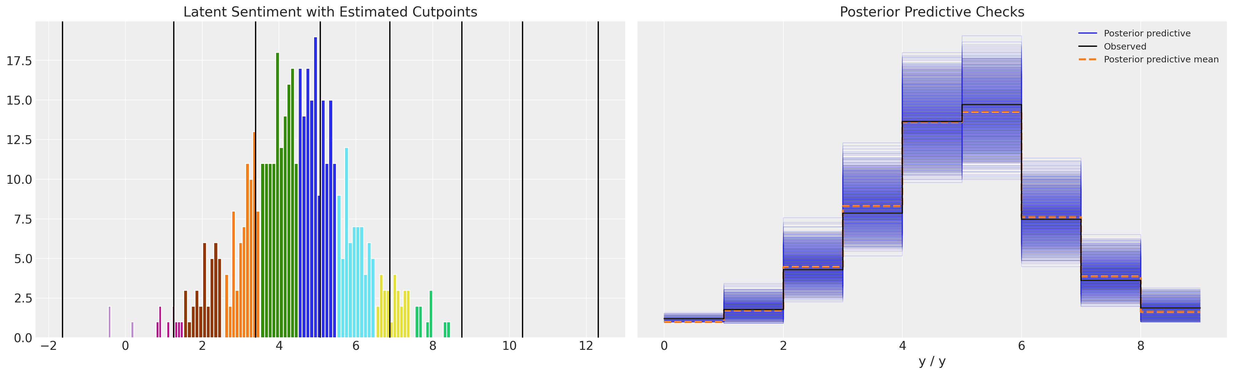
比较切点:正态先验与均匀先验#
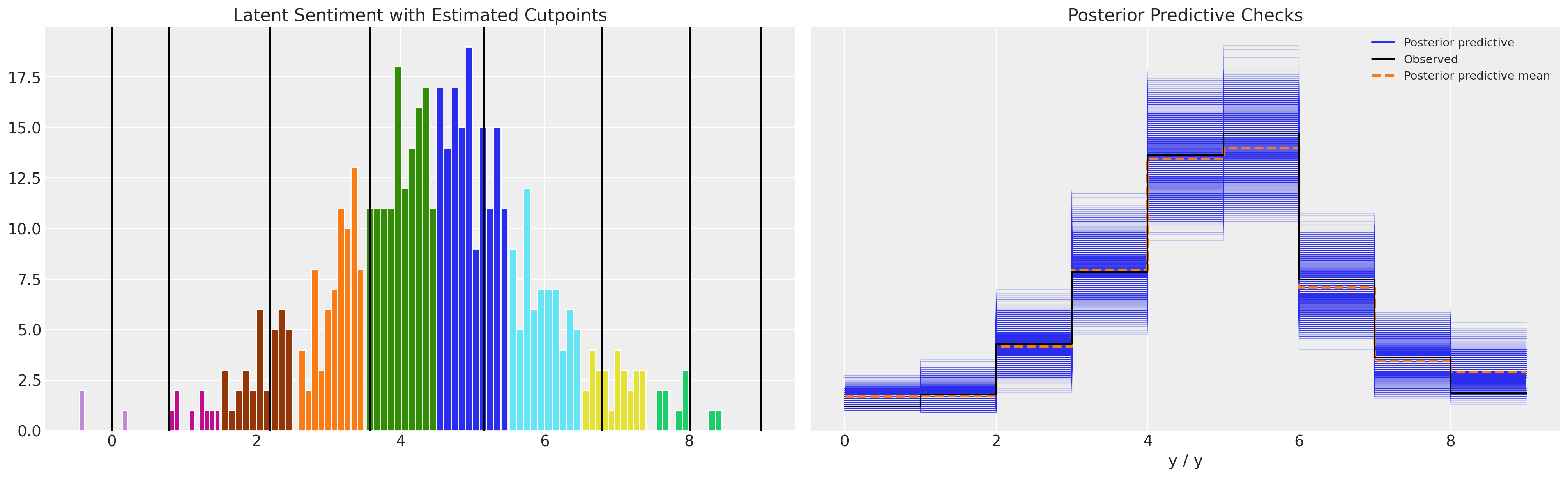
请注意,具有无约束截点的模型允许出现估计低于零的阈值。这在概念上没有太大意义,但可能导致足够合理的后验预测分布。
def plot_fit(idata):
    posterior = idata.posterior.stack(sample=("chain", "draw"))
    fig, axs = plt.subplots(1, 2, figsize=(20, 6))
    axs = axs.flatten()
    ax = axs[0]
    for i in range(K - 1):
        ax.axvline(posterior["cutpoints"][i].mean().values, color="k")
    for r in df["explicit_rating"].unique():
        temp = df[df["explicit_rating"] == r]
        ax.hist(temp["latent_rating"], ec="white")
    ax.set_title("Latent Sentiment with Estimated Cutpoints")
    axs[1].set_title("Posterior Predictive Checks")
    az.plot_ppc(idata, ax=axs[1])
    plt.show()


plot_fit(idata3)
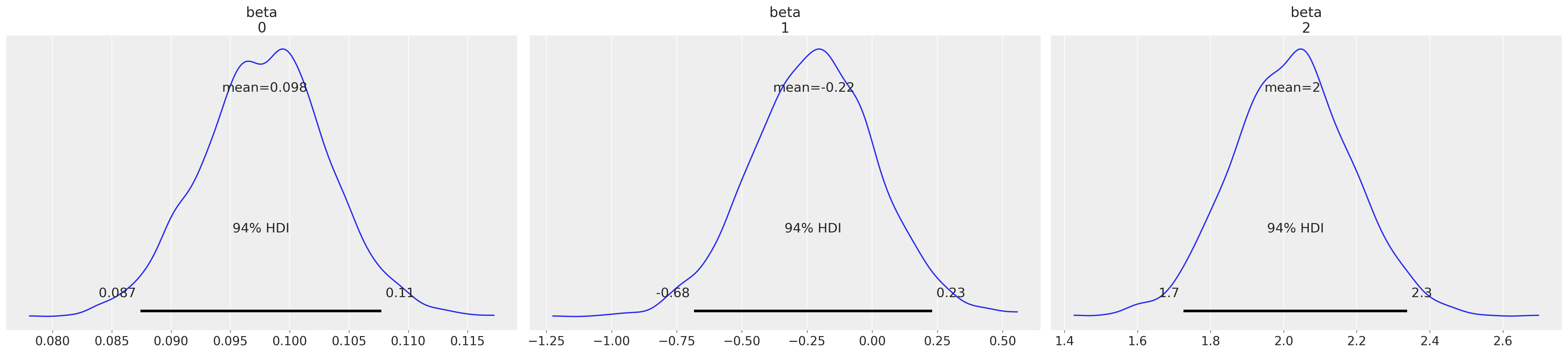
az.plot_posterior(idata3, var_names=["beta"]);
az.summary(idata3, var_names=["cutpoints"])
| mean | sd | hdi_3% | hdi_97% | mcse_mean | mcse_sd | ess_bulk | ess_tail | r_hat | |
|---|---|---|---|---|---|---|---|---|---|
| cutpoints[0] | -1.639 | 0.793 | -3.173 | -0.239 | 0.015 | 0.011 | 2810.0 | 2564.0 | 1.0 |
| cutpoints[1] | 1.262 | 0.464 | 0.409 | 2.139 | 0.007 | 0.005 | 4086.0 | 3251.0 | 1.0 |
| cutpoints[2] | 3.389 | 0.441 | 2.598 | 4.249 | 0.008 | 0.005 | 3252.0 | 3280.0 | 1.0 |
| cutpoints[3] | 5.074 | 0.466 | 4.179 | 5.941 | 0.009 | 0.006 | 2850.0 | 2614.0 | 1.0 |
| cutpoints[4] | 6.886 | 0.508 | 5.964 | 7.875 | 0.010 | 0.007 | 2558.0 | 2924.0 | 1.0 |
| cutpoints[5] | 8.765 | 0.563 | 7.664 | 9.800 | 0.011 | 0.008 | 2440.0 | 3031.0 | 1.0 |
| cutpoints[6] | 10.338 | 0.614 | 9.183 | 11.505 | 0.012 | 0.009 | 2475.0 | 2949.0 | 1.0 |
| cutpoints[7] | 12.316 | 0.722 | 11.030 | 13.758 | 0.014 | 0.010 | 2633.0 | 3016.0 | 1.0 |
虽然参数估计看起来合理,后验预测检查也似乎不错,但这里需要注意的是,切点不受有序尺度定义的约束。在上面的模型中,它们在0以下变化。
然而,如果我们查看带有约束Dirchlet先验的模型:
plot_fit(idata4)
az.plot_posterior(idata4, var_names=["beta"]);
再次,参数看起来合理,后验预测检查也是合理的。但现在,使用约束均匀先验分布在切点上,我们的估计切点符合有序尺度的定义。
az.summary(idata4, var_names=["cutpoints"])
/Users/nathanielforde/mambaforge/envs/pymc_examples_new/lib/python3.9/site-packages/arviz/stats/diagnostics.py:592: RuntimeWarning: invalid value encountered in double_scalars
  (between_chain_variance / within_chain_variance + num_samples - 1) / (num_samples)
| mean | sd | hdi_3% | hdi_97% | mcse_mean | mcse_sd | ess_bulk | ess_tail | r_hat | |
|---|---|---|---|---|---|---|---|---|---|
| cutpoints[0] | 0.000 | 0.000 | 0.000 | 0.000 | 0.000 | 0.000 | 4000.0 | 4000.0 | NaN |
| cutpoints[1] | 0.794 | 0.192 | 0.438 | 1.159 | 0.003 | 0.002 | 3170.0 | 2907.0 | 1.0 |
| cutpoints[2] | 2.195 | 0.192 | 1.827 | 2.544 | 0.003 | 0.002 | 4133.0 | 3275.0 | 1.0 |
| cutpoints[3] | 3.584 | 0.180 | 3.242 | 3.924 | 0.003 | 0.002 | 4267.0 | 3214.0 | 1.0 |
| cutpoints[4] | 5.161 | 0.179 | 4.827 | 5.494 | 0.003 | 0.002 | 4725.0 | 3299.0 | 1.0 |
| cutpoints[5] | 6.790 | 0.182 | 6.424 | 7.110 | 0.003 | 0.002 | 4758.0 | 3417.0 | 1.0 |
| cutpoints[6] | 8.012 | 0.163 | 7.706 | 8.312 | 0.002 | 0.002 | 5549.0 | 2791.0 | 1.0 |
| cutpoints[7] | 9.000 | 0.000 | 9.000 | 9.000 | 0.000 | 0.000 | 3945.0 | 3960.0 | 1.0 |
与Statsmodels的比较#
这种类型的模型也可以使用最大似然方法在频率学派的传统中进行估计。
modf_logit = OrderedModel.from_formula(
    "explicit_rating ~ salary + work_sat + work_from_home", df, distr="logit"
)
resf_logit = modf_logit.fit(method="bfgs")
resf_logit.summary()
Optimization terminated successfully.
         Current function value: 1.447704
         Iterations: 59
         Function evaluations: 65
         Gradient evaluations: 65
| Dep. Variable: | explicit_rating | Log-Likelihood: | -723.85 |
|---|---|---|---|
| Model: | OrderedModel | AIC: | 1470. |
| Method: | Maximum Likelihood | BIC: | 1516. |
| Date: | Thu, 01 Jun 2023 | ||
| Time: | 21:32:42 | ||
| No. Observations: | 500 | ||
| Df Residuals: | 489 | ||
| Df Model: | 11 |
| coef | std err | z | P>|z| | [0.025 | 0.975] | |
|---|---|---|---|---|---|---|
| salary | 0.1349 | 0.010 | 13.457 | 0.000 | 0.115 | 0.155 |
| work_sat | 0.0564 | 0.286 | 0.197 | 0.844 | -0.504 | 0.617 |
| work_from_home | 2.5985 | 0.206 | 12.590 | 0.000 | 2.194 | 3.003 |
| -0.0/1.0 | 0.2158 | 0.693 | 0.312 | 0.755 | -1.142 | 1.573 |
| 1.0/2.0 | 0.5127 | 0.332 | 1.543 | 0.123 | -0.138 | 1.164 |
| 2.0/3.0 | 0.6502 | 0.161 | 4.034 | 0.000 | 0.334 | 0.966 |
| 3.0/4.0 | 0.4962 | 0.108 | 4.598 | 0.000 | 0.285 | 0.708 |
| 4.0/5.0 | 0.6032 | 0.080 | 7.556 | 0.000 | 0.447 | 0.760 |
| 5.0/6.0 | 0.6399 | 0.076 | 8.474 | 0.000 | 0.492 | 0.788 |
| 6.0/7.0 | 0.4217 | 0.113 | 3.725 | 0.000 | 0.200 | 0.644 |
| 7.0/8.0 | 0.5054 | 0.186 | 2.712 | 0.007 | 0.140 | 0.871 |
我们还可以提取阈值或切点估计值,这些估计值与上述使用正态分布来表示潜在管理者评分的切点非常接近。
num_of_thresholds = 8
modf_logit.transform_threshold_params(resf_logit.params[-num_of_thresholds:])
array([       -inf,  0.21579015,  1.88552907,  3.80152819,  5.44399832,
        7.27200739,  9.16821716, 10.69274536, 12.35046331,         inf])
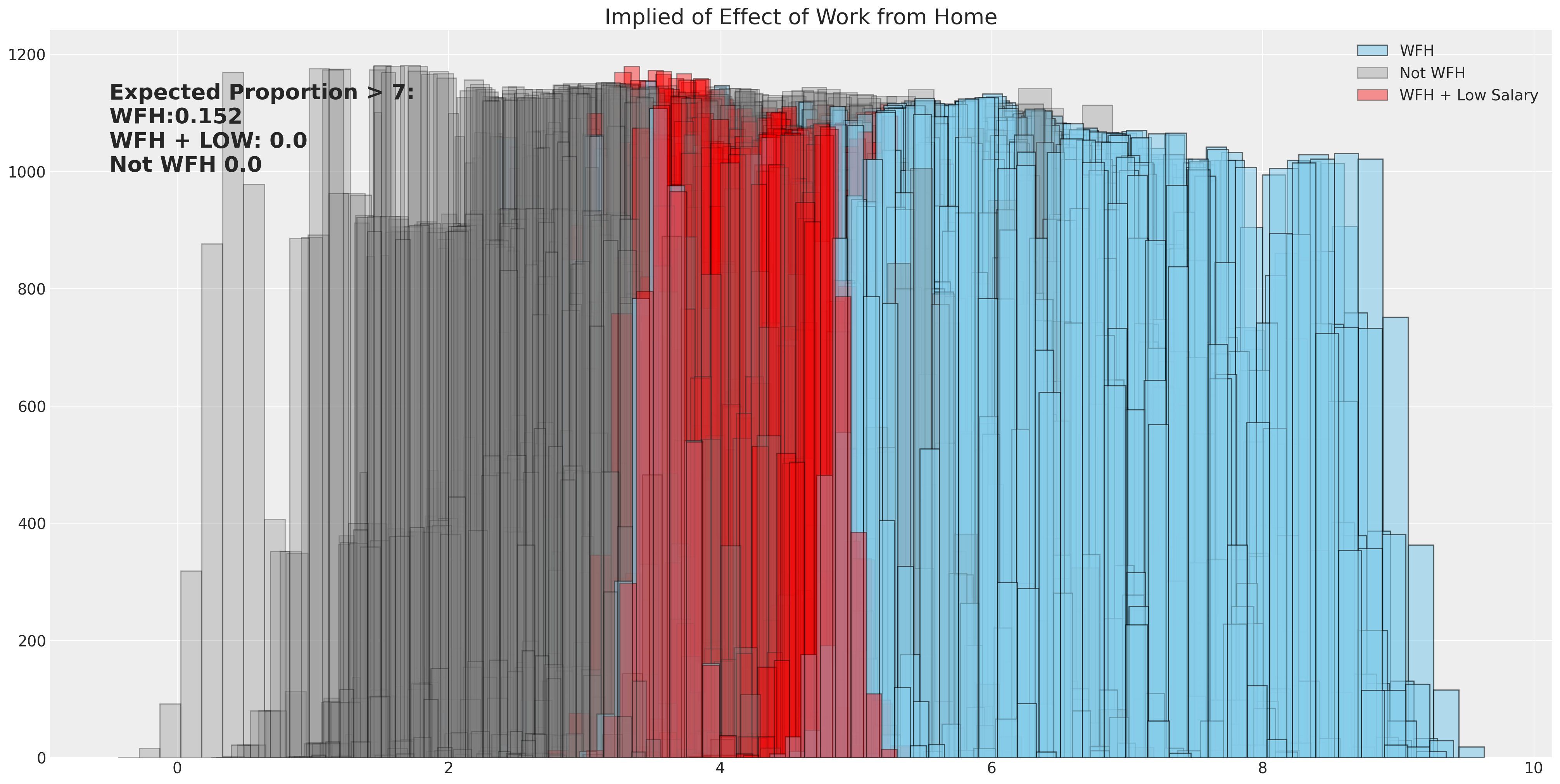
质询模型的含义#
当我们想要评估模型的影响时,我们可以使用数据生成方程的学习后验估计,来模拟在特定阈值分数下,调查结果的比例会是多少。这里我们允许在不同工作条件下,各种beta分布的完全不确定性得到体现,并测量给出经理评分高于7的员工比例。
betas_posterior = az.extract(idata4)["beta"]

fig, ax = plt.subplots(figsize=(20, 10))
calc_wfh = [
    df.iloc[i]["salary"] * betas_posterior[0, :]
    + df.iloc[i]["work_sat"] * betas_posterior[1, :]
    + 1 * betas_posterior[2, :]
    for i in range(500)
]
calc_not_wfh = [
    df.iloc[i]["salary"] * betas_posterior[0, :]
    + df.iloc[i]["work_sat"] * betas_posterior[1, :]
    + 0 * betas_posterior[2, :]
    for i in range(500)
]
sal = np.random.normal(25, 5, 500)
calc_wfh_and_low_sal = [
    sal[i] * betas_posterior[0, :]
    + df.iloc[i]["work_sat"] * betas_posterior[1, :]
    + 1 * betas_posterior[2, :]
    for i in range(500)
]

### Use implied threshold on latent score to predict proportion of ratings above 7
prop_wfh = np.sum([np.mean(calc_wfh[i].values) > 6.78 for i in range(500)]) / 500
prop_not_wfh = np.sum([np.mean(calc_not_wfh[i].values) > 6.78 for i in range(500)]) / 500
prop_wfh_low = np.sum([np.mean(calc_wfh_and_low_sal[i].values) > 6.78 for i in range(500)]) / 500

for i in range(500):
    if i == 499:
        ax.hist(calc_wfh[i], alpha=0.6, color="skyblue", ec="black", label="WFH")
        ax.hist(calc_not_wfh[i], alpha=0.3, color="grey", ec="black", label="Not WFH")
        ax.hist(
            calc_wfh_and_low_sal[i], alpha=0.4, color="red", ec="black", label="WFH + Low Salary"
        )
    else:
        ax.hist(calc_wfh[i], alpha=0.6, color="skyblue", ec="black")
        ax.hist(calc_wfh_and_low_sal[i], alpha=0.4, color="red", ec="black")
        ax.hist(calc_not_wfh[i], alpha=0.3, color="grey", ec="black")
ax.set_title("Implied of Effect of Work from Home", fontsize=20)
ax.annotate(
    f"Expected Proportion > 7: \nWFH:{prop_wfh} \nWFH + LOW: {prop_wfh_low} \nNot WFH {prop_not_wfh}",
    xy=(-0.5, 1000),
    fontsize=20,
    fontweight="bold",
)
ax.legend();
Liddell 和 Kruschke 的 IMDB 电影评分数据#
使用有序回归模型而不是依赖于替代模型规范有充分的理由。例如,将有序类别视为连续度量的诱惑将导致错误的推论。关于这一点的详细讨论可以在Liddell和Kruschke的论文[Liddell 和 Kruschke, 2018]中找到。我们将简要复制他们关于这种现象如何出现在电影评分数据分析中的例子。
try:
    movies = pd.read_csv("../data/MoviesData.csv")
except FileNotFoundError:
    movies = pd.DataFrame(pm.get_data("MoviesData.csv"))
def pivot_movie(row):
    row_ratings = row[["n1", "n2", "n3", "n4", "n5"]]
    totals = []
    for c, i in zip(row_ratings.index, range(5)):
        totals.append(row_ratings[c] * [i])
    totals = [item for sublist in totals for item in sublist]
    movie = [row["Descrip"]] * len(totals)
    id = [row["ID"]] * len(totals)
    return pd.DataFrame({"rating": totals, "movie": movie, "movie_id": id})


movies_by_rating = pd.concat([pivot_movie(movies.iloc[i]) for i in range(len(movies))])
movies_by_rating.reset_index(inplace=True, drop=True)
movies_by_rating.shape
(284671, 3)
movies_by_rating.sample(100).head()
| rating | movie | movie_id | |
|---|---|---|---|
| 169636 | 4 | The Man in the High Castle Season 1 | 23 |
| 218859 | 4 | The Man in the High Castle Season 1 | 23 |
| 252960 | 4 | Hunted Season 1 | 26 |
| 8304 | 1 | Room | 6 |
| 99958 | 4 | Sneaky Pete Season 1 | 19 |
def constrainedUniform(N, group, min=0, max=1):
    return pm.Deterministic(
        f"cutpoints_{group}",
        pt.concatenate(
            [
                np.ones(1) * min,
                pt.extra_ops.cumsum(pm.Dirichlet(f"cuts_unknown_{group}", a=np.ones(N - 2)))
                * (max - min)
                + min,
            ]
        ),
    )
我们将使用序数模型和度量模型来拟合这些数据。这将展示序数拟合在实质上更具说服力。
K = 5
movies_by_rating = movies_by_rating[movies_by_rating["movie_id"].isin([1, 2, 3, 4, 5, 6])]
indx, unique = pd.factorize(movies_by_rating["movie_id"])
priors = {"sigma": 1, "mu": [0, 1], "cut_mu": np.linspace(0, K, K - 1)}


def make_movies_model(ordered=False):
    with pm.Model() as model:
        for g in movies_by_rating["movie_id"].unique():
            if ordered:
                cutpoints = constrainedUniform(K, g, 0, K - 1)
                mu = pm.Normal(f"mu_{g}", 0, 1)
                y_ = pm.OrderedLogistic(
                    f"y_{g}",
                    cutpoints=cutpoints,
                    eta=mu,
                    observed=movies_by_rating[movies_by_rating["movie_id"] == g].rating.values,
                )
            else:
                mu = pm.Normal(f"mu_{g}", 0, 1)
                sigma = pm.HalfNormal(f"sigma_{g}", 1)
                y_ = pm.Normal(
                    f"y_{g}",
                    mu,
                    sigma,
                    observed=movies_by_rating[movies_by_rating["movie_id"] == g].rating.values,
                )

        idata = pm.sample_prior_predictive()
        idata.extend(pm.sample(nuts_sampler="numpyro", idata_kwargs={"log_likelihood": True}))
        idata.extend(pm.sample_posterior_predictive(idata))
    return idata, model


idata_ordered, model_ordered = make_movies_model(ordered=True)
idata_normal_metric, model_normal_metric = make_movies_model(ordered=False)
Show code cell output
Sampling: [cuts_unknown_1, cuts_unknown_2, cuts_unknown_3, cuts_unknown_4, cuts_unknown_5, cuts_unknown_6, mu_1, mu_2, mu_3, mu_4, mu_5, mu_6, y_1, y_2, y_3, y_4, y_5, y_6]
/Users/nathanielforde/mambaforge/envs/pymc_examples_new/lib/python3.9/site-packages/pymc/sampling/mcmc.py:243: UserWarning: Use of external NUTS sampler is still experimental
  warnings.warn("Use of external NUTS sampler is still experimental", UserWarning)
Compiling...
Compilation time =  0:00:04.998186
Sampling...
Sampling time =  0:00:09.785681
Transforming variables...
Transformation time =  0:00:00.432907
Computing Log Likelihood...
Sampling: [mu_1, mu_2, mu_3, mu_4, mu_5, mu_6, sigma_1, sigma_2, sigma_3, sigma_4, sigma_5, sigma_6, y_1, y_2, y_3, y_4, y_5, y_6]
/Users/nathanielforde/mambaforge/envs/pymc_examples_new/lib/python3.9/site-packages/pymc/sampling/mcmc.py:243: UserWarning: Use of external NUTS sampler is still experimental
  warnings.warn("Use of external NUTS sampler is still experimental", UserWarning)
Compiling...
Compilation time =  0:00:01.414912
Sampling...
Sampling time =  0:00:05.203627
Transforming variables...
Transformation time =  0:00:00.008429
Computing Log Likelihood...
后验预测拟合:正态度量模型#
这是一个对六部电影评分数据的可怕拟合。
axs = az.plot_ppc(idata_normal_metric)
axs = axs.flatten()
for ax in axs:
    ax.set_xlim(0, 5);
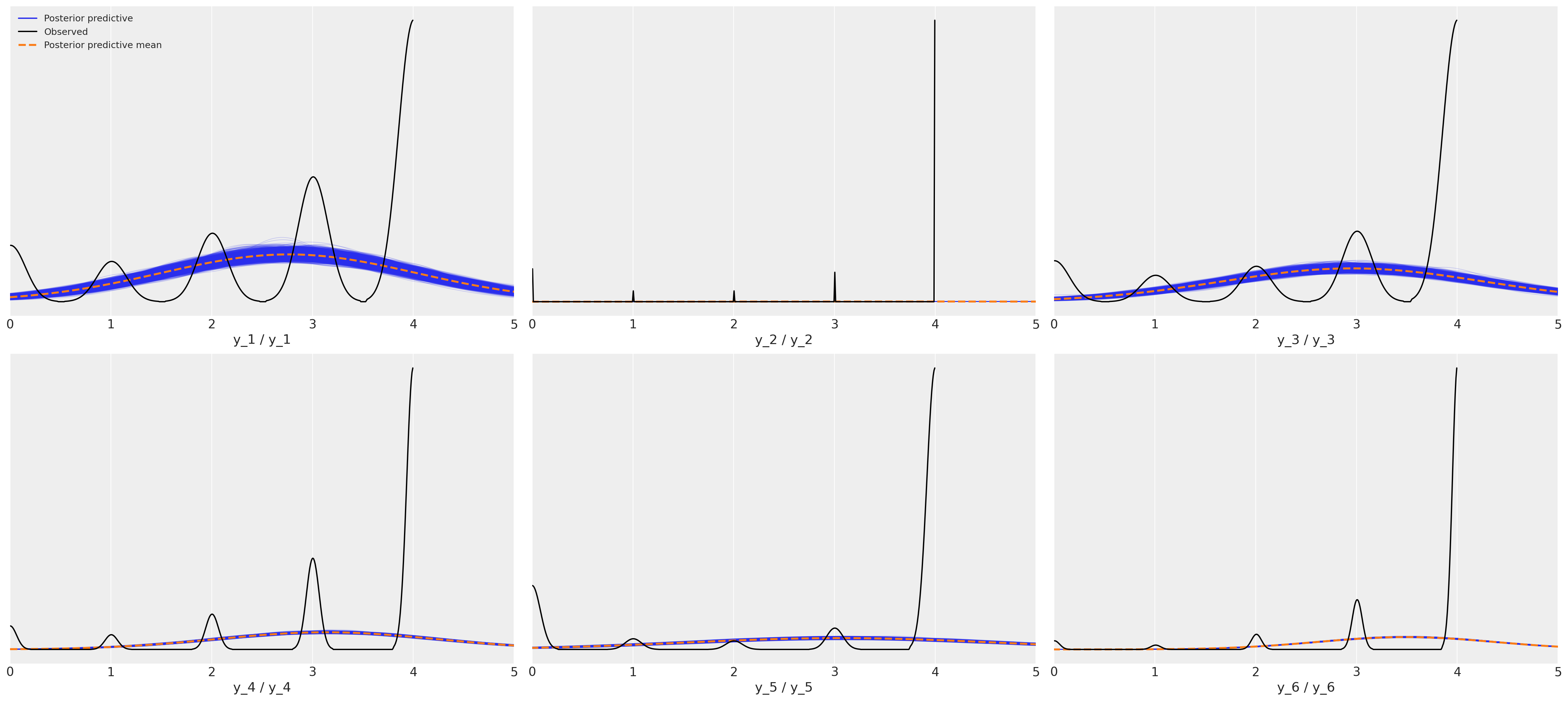
后验预测拟合:有序响应模型#
这显示了六部电影中每一部的更合适的拟合。
az.plot_ppc(idata_ordered);
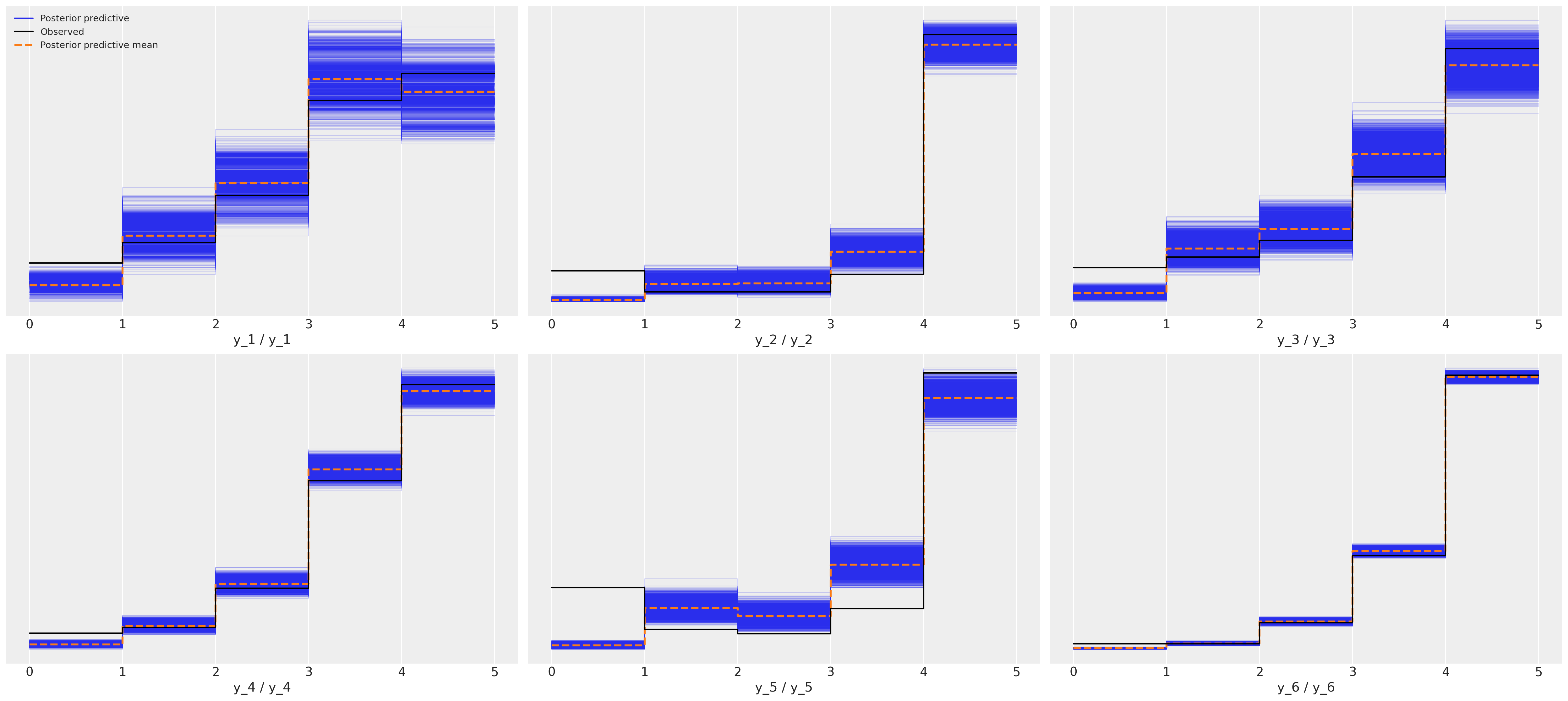
由于这是真实数据,我们不知道真实的数据生成过程,因此无法确定哪个是正确的模型,但我希望你会同意后验预测检查强烈支持有序分类拟合是一个更强候选者的说法。这里更简单的观点是,度量模型的推论是错误的,如果我们希望对可能影响电影评分的因素做出合理的推断,那么我们最好确保不要通过选择不恰当的似然函数在模型构建中引入噪声。
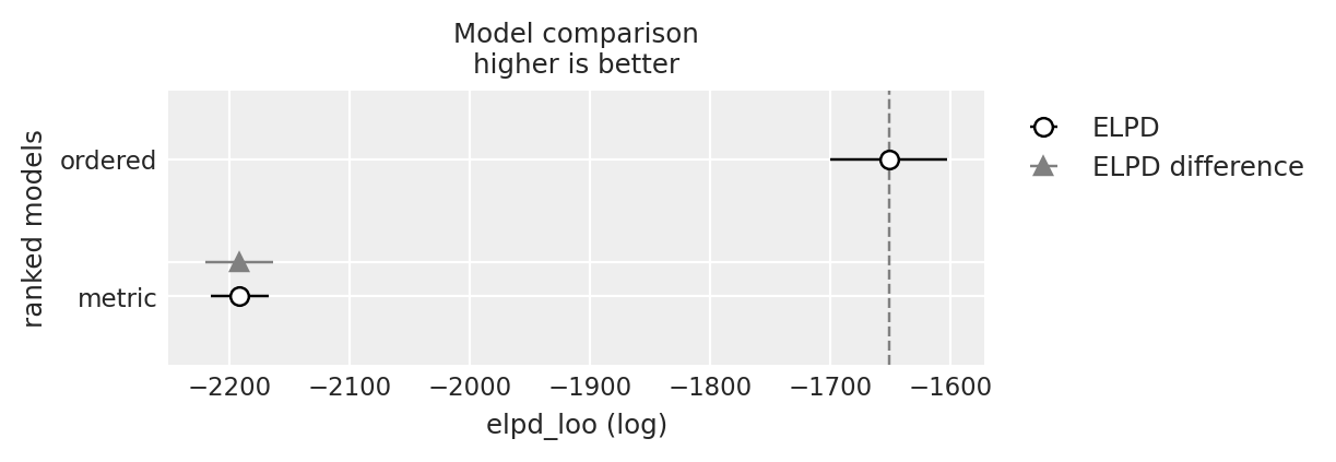
比较模型拟合#
y_5_compare = az.compare({"ordered": idata_ordered, "metric": idata_normal_metric}, var_name="y_5")
y_5_compare
| rank | elpd_loo | p_loo | elpd_diff | weight | se | dse | warning | scale | |
|---|---|---|---|---|---|---|---|---|---|
| ordered | 0 | -1651.276933 | 3.496302 | 0.000000 | 1.000000e+00 | 48.836869 | 0.000000 | False | log |
| metric | 1 | -2191.541142 | 2.062035 | 540.264208 | 5.153936e-09 | 24.050997 | 28.196537 | False | log |
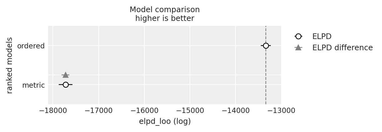
y_6_compare = az.compare({"ordered": idata_ordered, "metric": idata_normal_metric}, var_name="y_6")
y_6_compare
| rank | elpd_loo | p_loo | elpd_diff | weight | se | dse | warning | scale | |
|---|---|---|---|---|---|---|---|---|---|
| ordered | 0 | -13339.249536 | 3.100333 | 0.000000 | 1.0 | 110.330929 | 0.000000 | False | log |
| metric | 1 | -17723.156659 | 4.154765 | 4383.907122 | 0.0 | 148.655963 | 85.797241 | False | log |
az.plot_compare(y_5_compare)
<Axes: title={'center': 'Model comparison\nhigher is better'}, xlabel='elpd_loo (log)', ylabel='ranked models'>
az.plot_compare(y_6_compare)
<Axes: title={'center': 'Model comparison\nhigher is better'}, xlabel='elpd_loo (log)', ylabel='ranked models'>
比较模型之间的推理#
除了预测拟合结果外,不同建模选择所得到的推论也存在相当大的差异。想象一下,如果你是一位电影制片人,正在考虑是否要制作续集,那么相对于竞争对手基准的相对电影表现评分可能是这一决策的关键因素,而分析师选择的模型差异可能会对这一选择产生重大影响。
mosaic = """
AC
DE
BB
"""
fig, axs = plt.subplot_mosaic(mosaic, figsize=(15, 7))
axs = [axs[k] for k in axs.keys()]
axs
ordered_5 = az.extract(idata_ordered.posterior_predictive)["y_5"].mean(axis=0)
ordered_6 = az.extract(idata_ordered.posterior_predictive)["y_6"].mean(axis=0)
diff = ordered_5 - ordered_6
metric_5 = az.extract(idata_normal_metric.posterior_predictive)["y_5"].mean(axis=0)
metric_6 = az.extract(idata_normal_metric.posterior_predictive)["y_6"].mean(axis=0)
diff1 = metric_5 - metric_6
axs[0].hist(ordered_5, bins=30, ec="white", color="slateblue", label="Ordered Fit Movie 5")
axs[4].plot(
    az.hdi(diff.unstack())["x"].values, [1, 1], "o-", color="slateblue", label="Ordered Fits"
)
axs[4].plot(
    az.hdi(diff1.unstack())["x"].values, [1.2, 1.2], "o-", color="magenta", label="Metric Fits"
)
axs[2].hist(ordered_6, bins=30, ec="white", color="slateblue", label="Ordered Fit Movie 6")
axs[3].hist(metric_5, ec="white", label="Metric Fit Movie 5", bins=30, color="magenta")
axs[1].hist(metric_6, ec="white", label="Metric Fit Movie 6", bins=30, color="magenta")
axs[4].set_title("Implied Differences Between the \n Expected Rating")
axs[4].set_ylim(0.8, 1.4)
axs[4].set_yticks([])
axs[0].set_title("Expected Posterior Predictive Estimate \n for Movies Ordered Fits")
axs[1].set_title("Expected Posterior Predictive Estimate \n for Movie Metric Fits")
axs[4].set_xlabel("Difference between Movie 5 and 6")
axs[1].legend()
axs[0].legend()
axs[2].legend()
axs[3].legend()
axs[4].legend();
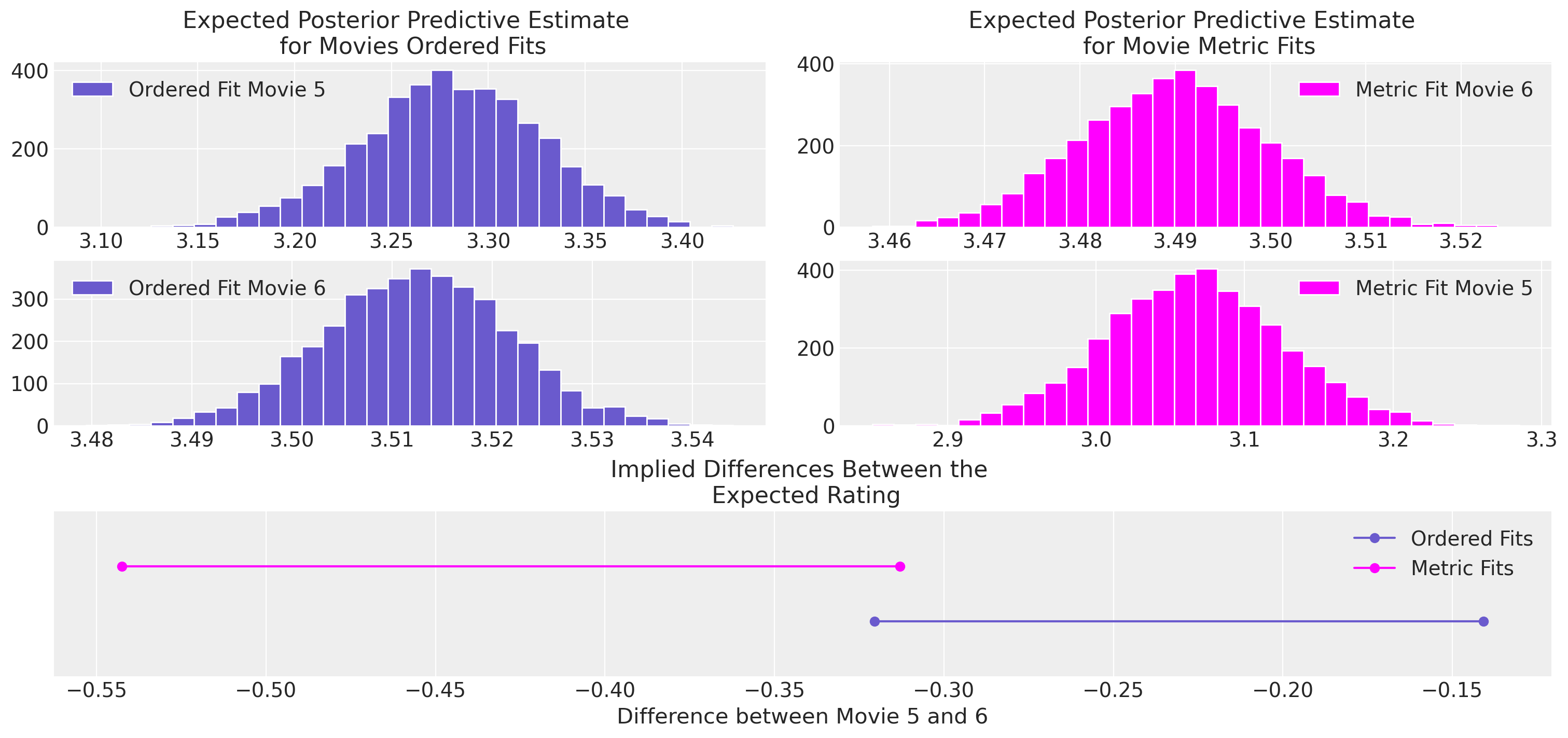
在决定将一部电影投入制作时,涉及到的资金可能高达数百万美元。这项投资的回报至少部分取决于电影的受欢迎程度,而这种受欢迎程度既可以通过烂番茄和IMDB的评分来衡量,也可以受到这些评分的影响。因此,理解不同电影的相对受欢迎程度可以通过好莱坞转移大量资金,这里所暗示的差异确实很重要。类似的考虑也适用于考虑更重要的评分标准,这些标准用于衡量幸福和抑郁程度。
结论#
在本笔记本中,我们了解了如何使用PyMC构建序数回归模型,并通过将序数结果解释为潜在连续现象的离散结果来激励建模练习。我们看到了不同的模型规范如何生成对模型参数的更易或更难解释的估计。我们还比较了序数回归方法与对序数数据的更简单的回归方法。结果强烈表明,序数回归避免了使用简单方法时出现的一些推断陷阱。此外,我们还展示了贝叶斯建模工作流程的灵活性可以提供对模型错误指定风险的保证,使其成为分析序数数据的可行且有吸引力的方法。
参考资料#
Torrin M. Liddell 和 John K. Kruschke。使用度量模型分析有序数据:可能会出什么问题?实验社会心理学杂志,2018年。
水印#
%load_ext watermark
%watermark -n -u -v -iv -w -p pytensor
Last updated: Thu Jun 01 2023

Python implementation: CPython
Python version       : 3.9.16
IPython version      : 8.11.0

pytensor: 2.11.1

numpy      : 1.23.5
arviz      : 0.15.1
pytensor   : 2.11.1
statsmodels: 0.13.5
pandas     : 1.5.3
pymc       : 5.3.0
matplotlib : 3.7.1

Watermark: 2.3.1
许可证声明#
本示例库中的所有笔记本均在MIT许可证下提供,该许可证允许修改和重新分发,前提是保留版权和许可证声明。
引用 PyMC 示例#
要引用此笔记本,请使用Zenodo为pymc-examples仓库提供的DOI。
重要
许多笔记本是从其他来源改编的:博客、书籍……在这种情况下,您应该引用原始来源。
同时记得引用代码中使用的相关库。
这是一个BibTeX的引用模板:
@incollection{citekey,
  author    = "<notebook authors, see above>",
  title     = "<notebook title>",
  editor    = "PyMC Team",
  booktitle = "PyMC examples",
  doi       = "10.5281/zenodo.5654871"
}
渲染后可能看起来像: