LKJ Cholesky 协方差先验用于多元正态模型#
虽然逆Wishart分布是多元正态分布协方差矩阵的共轭先验,但它并不非常适合现代贝叶斯计算方法。因此,在为多元正态分布的协方差矩阵建模时,建议使用LKJ先验。
为了说明使用LKJ分布建模协方差,我们首先生成一个二维正态分布的样本数据集。
import arviz as az
import numpy as np
import pymc as pm

from matplotlib import pyplot as plt
from matplotlib.lines import Line2D
from matplotlib.patches import Ellipse

print(f"Running on PyMC v{pm.__version__}")
Running on PyMC v5.9.0
%config InlineBackend.figure_format = 'retina'
RANDOM_SEED = 8927
rng = np.random.default_rng(RANDOM_SEED)
az.style.use("arviz-darkgrid")
N = 10000

mu_actual = np.array([1.0, -2.0])
sigmas_actual = np.array([0.7, 1.5])
Rho_actual = np.matrix([[1.0, -0.4], [-0.4, 1.0]])

Sigma_actual = np.diag(sigmas_actual) * Rho_actual * np.diag(sigmas_actual)

x = rng.multivariate_normal(mu_actual, Sigma_actual, size=N)
Sigma_actual
matrix([[ 0.49, -0.42],
        [-0.42,  2.25]])
var, U = np.linalg.eig(Sigma_actual)
angle = 180.0 / np.pi * np.arccos(np.abs(U[0, 0]))

fig, ax = plt.subplots(figsize=(8, 6))

e = Ellipse(mu_actual, 2 * np.sqrt(5.991 * var[0]), 2 * np.sqrt(5.991 * var[1]), angle=angle)
e.set_alpha(0.5)
e.set_facecolor("C0")
e.set_zorder(10)
ax.add_artist(e)

ax.scatter(x[:, 0], x[:, 1], c="k", alpha=0.05, zorder=11)
ax.set_xlabel("y")
ax.set_ylabel("z")

rect = plt.Rectangle((0, 0), 1, 1, fc="C0", alpha=0.5)
ax.legend([rect], ["95% density region"], loc=2);
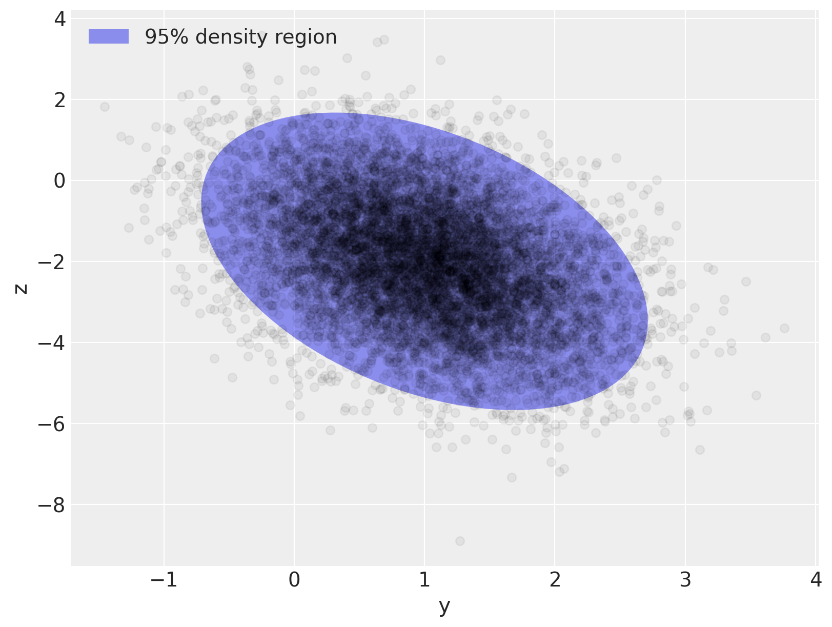
多元正态模型的抽样分布为 \(\mathbf{x} \sim N(\mu, \Sigma)\),其中 \(\Sigma\) 是抽样分布的协方差矩阵,且 \(\Sigma_{ij} = \textrm{Cov}(x_i, x_j)\)。该分布的密度为
LKJ 分布提供了一个关于相关矩阵的先验,\(\mathbf{C} = \textrm{Corr}(x_i, x_j)\),它与每个分量的标准差的先验结合,诱导出一个关于协方差矩阵的先验,\(\Sigma\)。由于反转 \(\Sigma\) 在数值上不稳定且效率低下,因此使用 \(\Sigma\) 的 Cholesky 分解,\(\Sigma = \mathbf{L} \mathbf{L}^{\top}\),其中 \(\mathbf{L}\) 是一个下三角矩阵,在计算上是有优势的。这种分解允许使用回代法计算项 \((\mathbf{x} - \mu)^{\top} \Sigma^{-1} (\mathbf{x} - \mu)\),这比直接矩阵求逆在数值上更稳定且更高效。
PyMC 支持通过 pymc.LKJCholeskyCov 分布对协方差矩阵的 Cholesky 分解使用 LKJ 先验。该分布具有参数 n 和 sd_dist,分别表示观测值的维度 \(\mathbf{x}\) 和分量标准差的 PyMC 分布。它还具有一个超参数 eta,用于控制 \(\mathbf{x}\) 分量之间的相关性程度。LKJ 分布具有密度 \(f(\mathbf{C}\ |\ \eta) \propto |\mathbf{C}|^{\eta - 1}\),因此 \(\eta = 1\) 会导致相关矩阵上的均匀分布,而随着 \(\eta \to \infty\),分量之间的相关性幅度会减小。
在这个例子中,我们使用 \(\textrm{Exponential}(1.0)\) 先验来建模标准差,并将相关矩阵建模为 \(\mathbf{C} \sim \textrm{LKJ}(\eta = 2)\)。
with pm.Model() as m:
    packed_L = pm.LKJCholeskyCov(
        "packed_L", n=2, eta=2.0, sd_dist=pm.Exponential.dist(1.0, shape=2), compute_corr=False
    )
由于\(\Sigma\)的Cholesky分解是下三角的,LKJCholeskyCov仅存储对角线和次对角线项,以提高效率:
packed_L.eval()
array([ 2.60423567, -1.28344686, 0.65139719])
我们使用 expand_packed_triangular 将这个向量转换为下三角矩阵 \(\mathbf{L}\),它出现在 Cholesky 分解 \(\Sigma = \mathbf{L} \mathbf{L}^{\top}\) 中。
with m:
    L = pm.expand_packed_triangular(2, packed_L)
    Sigma = L.dot(L.T)

L.eval().shape
(2, 2)
然而,通常情况下,您会对相关矩阵和标准差的后验分布感兴趣,而不是对后验的Cholesky协方差矩阵本身感兴趣。为什么?因为相关性和标准差更容易解释,并且在模型中通常具有科学意义。从PyMC v4开始,compute_corr参数默认设置为True,这将返回一个由Cholesky分解、相关矩阵和标准差组成的元组。
coords = {"axis": ["y", "z"], "axis_bis": ["y", "z"], "obs_id": np.arange(N)}
with pm.Model(coords=coords) as model:
    chol, corr, stds = pm.LKJCholeskyCov(
        "chol", n=2, eta=2.0, sd_dist=pm.Exponential.dist(1.0, shape=2)
    )
    cov = pm.Deterministic("cov", chol.dot(chol.T), dims=("axis", "axis_bis"))
为了完成我们的模型,我们在\(\mu\)上放置了独立、弱正则化的先验,\(N(0, 1.5),\):
with model:
    mu = pm.Normal("mu", 0.0, sigma=1.5, dims="axis")
    obs = pm.MvNormal("obs", mu, chol=chol, observed=x, dims=("obs_id", "axis"))
我们使用NUTS从这个模型中采样,并将轨迹传递给arviz进行汇总:
with model:
    trace = pm.sample(
        random_seed=rng,
        idata_kwargs={"dims": {"chol_stds": ["axis"], "chol_corr": ["axis", "axis_bis"]}},
    )
az.summary(trace, var_names="~chol", round_to=2)
Auto-assigning NUTS sampler...
Initializing NUTS using jitter+adapt_diag...
Multiprocess sampling (4 chains in 4 jobs)
NUTS: [chol, mu]
Sampling 4 chains for 1_000 tune and 1_000 draw iterations (4_000 + 4_000 draws total) took 31 seconds.
/home/erik/mambaforge/envs/pymc_examples/lib/python3.11/site-packages/arviz/stats/diagnostics.py:592: RuntimeWarning: invalid value encountered in scalar divide
  (between_chain_variance / within_chain_variance + num_samples - 1) / (num_samples)
| mean | sd | hdi_3% | hdi_97% | mcse_mean | mcse_sd | ess_bulk | ess_tail | r_hat | |
|---|---|---|---|---|---|---|---|---|---|
| mu[y] | 1.00 | 0.01 | 0.99 | 1.01 | 0.0 | 0.0 | 4121.45 | 3183.18 | 1.0 |
| mu[z] | -2.01 | 0.01 | -2.04 | -1.99 | 0.0 | 0.0 | 4649.42 | 3413.88 | 1.0 |
| chol_corr[y, y] | 1.00 | 0.00 | 1.00 | 1.00 | 0.0 | 0.0 | 4000.00 | 4000.00 | NaN |
| chol_corr[y, z] | -0.40 | 0.01 | -0.42 | -0.39 | 0.0 | 0.0 | 4986.71 | 3442.98 | 1.0 |
| chol_corr[z, y] | -0.40 | 0.01 | -0.42 | -0.39 | 0.0 | 0.0 | 4986.71 | 3442.98 | 1.0 |
| chol_corr[z, z] | 1.00 | 0.00 | 1.00 | 1.00 | 0.0 | 0.0 | 3458.80 | 3722.51 | 1.0 |
| chol_stds[y] | 0.70 | 0.01 | 0.69 | 0.71 | 0.0 | 0.0 | 5112.65 | 3038.55 | 1.0 |
| chol_stds[z] | 1.49 | 0.01 | 1.47 | 1.51 | 0.0 | 0.0 | 5330.27 | 3156.89 | 1.0 |
| cov[y, y] | 0.49 | 0.01 | 0.48 | 0.51 | 0.0 | 0.0 | 5112.65 | 3038.55 | 1.0 |
| cov[y, z] | -0.42 | 0.01 | -0.44 | -0.40 | 0.0 | 0.0 | 4320.77 | 3391.79 | 1.0 |
| cov[z, y] | -0.42 | 0.01 | -0.44 | -0.40 | 0.0 | 0.0 | 4320.77 | 3391.79 | 1.0 |
| cov[z, z] | 2.23 | 0.03 | 2.17 | 2.28 | 0.0 | 0.0 | 5330.27 | 3156.89 | 1.0 |
采样进行得很顺利:没有分歧,且r-hat值良好(除了相关矩阵的对角元素 - 不过,这些并不令人担忧,因为对于每个链的每个样本,它们应该等于1,而常数值的方差是未定义的。如果对角元素之一有r_hat定义,这很可能是由于极小的数值误差)。
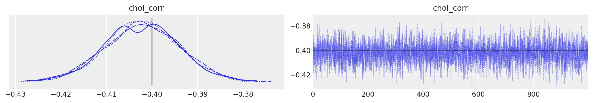
你也可以看到采样器恢复了真实的均值、相关性和标准差。通常,这在图表中会更加清晰:
az.plot_trace(
    trace,
    var_names="chol_corr",
    coords={"axis": "y", "axis_bis": "z"},
    lines=[("chol_corr", {}, Rho_actual[0, 1])],
);
az.plot_trace(
    trace,
    var_names=["~chol", "~chol_corr"],
    compact=True,
    lines=[
        ("mu", {}, mu_actual),
        ("cov", {}, Sigma_actual),
        ("chol_stds", {}, sigmas_actual),
    ],
);
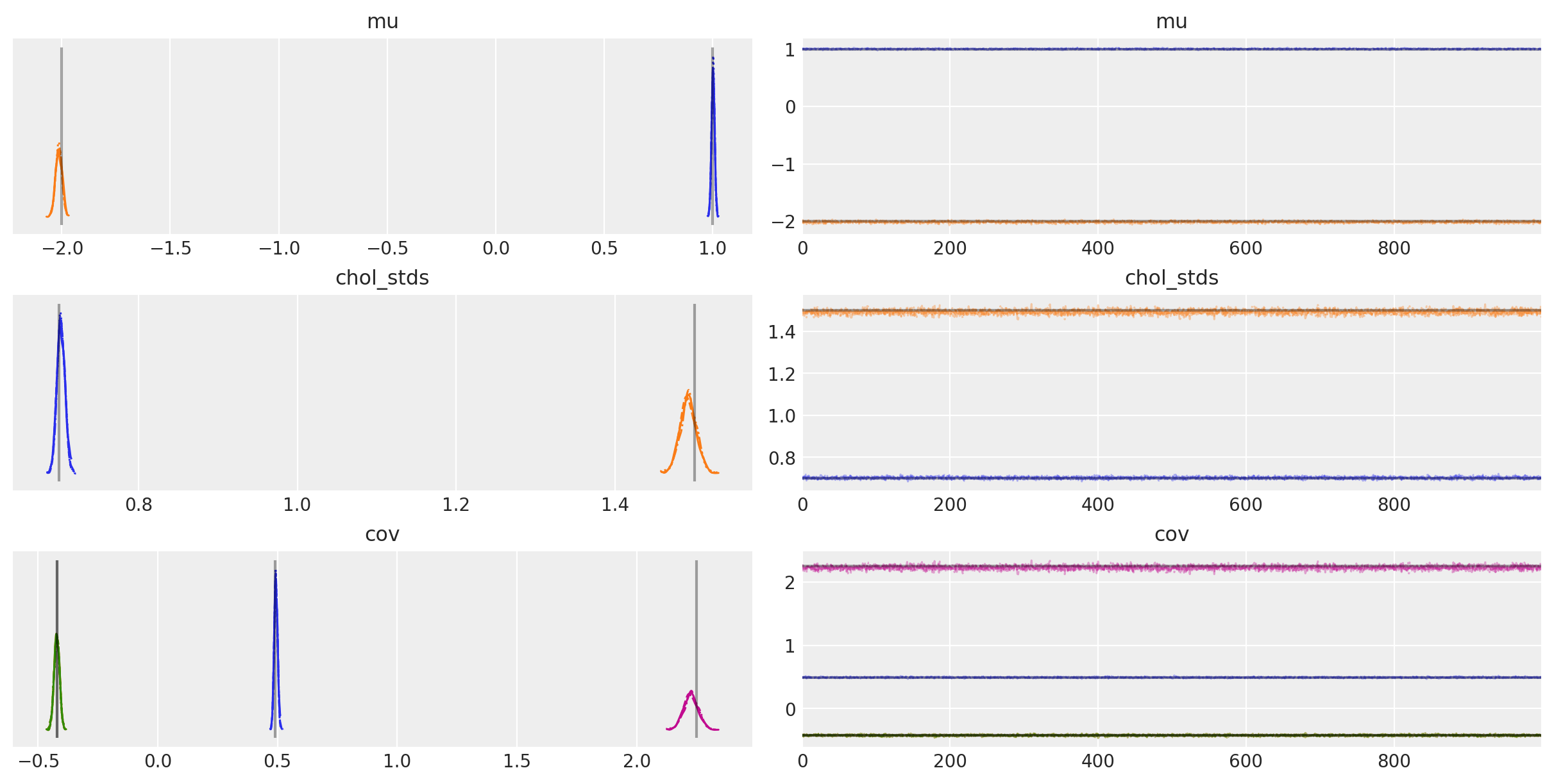
后验期望值非常接近每个分量的真实值!具体有多接近?让我们计算\(\mu\)和\(\Sigma\)的接近百分比:
mu_post = trace.posterior["mu"].mean(("chain", "draw")).values
(1 - mu_post / mu_actual).round(2)
array([-0. , -0.01])
Sigma_post = trace.posterior["cov"].mean(("chain", "draw")).values
(1 - Sigma_post / Sigma_actual).round(2)
array([[-0.01, -0.  ],
       [-0.  ,  0.01]])
因此,后验均值在\(\mu\)和\(\Sigma\)的真实值的1%以内。
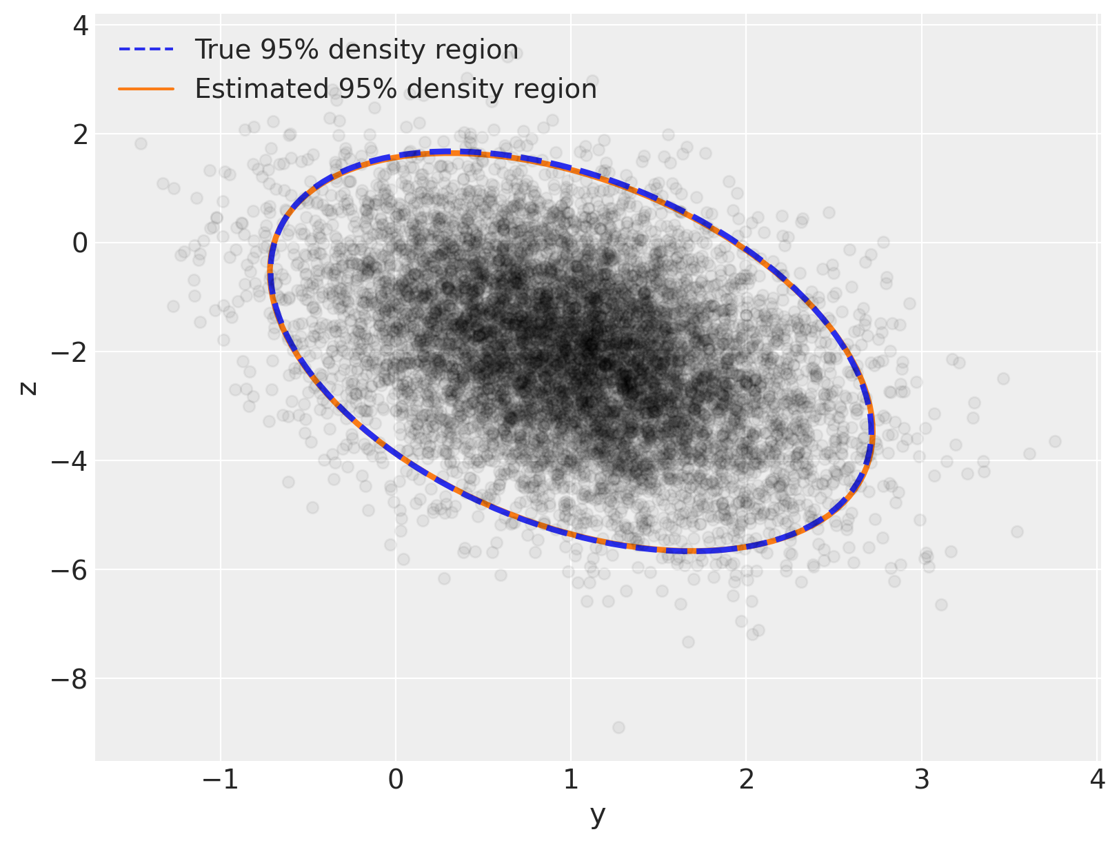
现在让我们复制我们在开始时绘制的图表,但让我们在真实分布的顶部叠加后验分布——你会看到两者之间有非常好的视觉一致性:
var_post, U_post = np.linalg.eig(Sigma_post)
angle_post = 180.0 / np.pi * np.arccos(np.abs(U_post[0, 0]))

fig, ax = plt.subplots(figsize=(8, 6))

e = Ellipse(
    mu_actual,
    2 * np.sqrt(5.991 * var[0]),
    2 * np.sqrt(5.991 * var[1]),
    angle=angle,
    linewidth=3,
    linestyle="dashed",
)
e.set_edgecolor("C0")
e.set_zorder(11)
e.set_fill(False)
ax.add_artist(e)

e_post = Ellipse(
    mu_post,
    2 * np.sqrt(5.991 * var_post[0]),
    2 * np.sqrt(5.991 * var_post[1]),
    angle=angle_post,
    linewidth=3,
)
e_post.set_edgecolor("C1")
e_post.set_zorder(10)
e_post.set_fill(False)
ax.add_artist(e_post)

ax.scatter(x[:, 0], x[:, 1], c="k", alpha=0.05, zorder=11)
ax.set_xlabel("y")
ax.set_ylabel("z")

line = Line2D([], [], color="C0", linestyle="dashed", label="True 95% density region")
line_post = Line2D([], [], color="C1", label="Estimated 95% density region")
ax.legend(
    handles=[line, line_post],
    loc=2,
);
%load_ext watermark
%watermark -n -u -v -iv -w -p pytensor,xarray
Last updated: Thu Oct 12 2023

Python implementation: CPython
Python version       : 3.11.6
IPython version      : 8.16.1

pytensor: 2.17.1
xarray  : 2023.9.0

numpy     : 1.25.2
matplotlib: 3.8.0
pymc      : 5.9.0
arviz     : 0.16.1

Watermark: 2.4.3