离散变量的自动边缘化#

PyMC非常适合用于对具有离散潜在变量的模型进行采样。但如果你坚持只使用NUTS采样器，你需要以某种方式消除离散变量。最好的方法是边缘化它们，这样你可以受益于Rao-Blackwell定理，并获得参数的较低方差估计。

形式上，这个论点是这样的，采样器可以理解为近似期望值 \(\mathbb{E}_{p(x, z)}[f(x, z)]\) 对于某个函数 \(f\) 相对于分布 \(p(x, z)\)。根据全期望定律，我们知道

\[ \mathbb{E}_{p(x, z)}[f(x, z)] = \mathbb{E}_{p(z)}\left[\mathbb{E}_{p(x \mid z)}\left[f(x, z)\right]\right] \]

令 \(g(z) = \mathbb{E}_{p(x \mid z)}\left[f(x, z)\right]\)，根据全变差定律，我们知道

\[ \mathbb{V}_{p(x, z)}[f(x, z)] = \mathbb{V}_{p(z)}[g(z)] + \mathbb{E}_{p(z)}\left[\mathbb{V}_{p(x \mid z)}\left[f(x, z)\right]\right] \]

因为期望值是针对方差计算的，所以它必须始终为正，因此我们知道

\[ \mathbb{V}_{p(x, z)}[f(x, z)] \geq \mathbb{V}_{p(z)}[g(z)] \]

直观地说，在模型中边缘化变量可以让您使用 \(g\) 而不是 \(f\)。这种较低的方差最直接体现在较低的蒙特卡罗标准误差（mcse），间接体现在通常较高的有效样本量（ESS）。

不幸的是，进行这种计算通常是繁琐且不直观的。幸运的是，pymc-experimental 现在支持自动完成这项工作！

import arviz as az
import matplotlib.pyplot as plt
import numpy as np
import pandas as pd
import pymc as pm
import pytensor.tensor as pt

注意

本笔记本使用了不是 PyMC 依赖项的库，因此需要专门安装这些库才能运行此笔记本。打开下面的下拉菜单以获取更多指导。

import pymc_experimental as pmx

%config InlineBackend.figure_format = 'retina'  # high resolution figures
az.style.use("arviz-darkgrid")
rng = np.random.default_rng(32)

作为一个激励性的例子，考虑一个高斯混合模型

高斯混合模型#

有两种方法可以指定相同的模型。一种是明确选择混合的方式。

mu = pt.as_tensor([-2.0, 2.0])

with pmx.MarginalModel() as explicit_mixture:
    idx = pm.Bernoulli("idx", 0.7)
    y = pm.Normal("y", mu=mu[idx], sigma=1.0)

plt.hist(pm.draw(y, draws=2000, random_seed=rng), bins=30, rwidth=0.9);

../_images/b9aa9d3c433d8157468cb50da64ed94ca24a2cf550e04e3f3cb95c6c81e6c714.png

另一种方法是使用内置的 NormalMixture 分布。在这里，混合分配在我们的模型中不是一个显式变量。第一个模型除了使用 pmx.MarginalModel 而不是 pm.Model 进行初始化之外，并没有什么特别之处。这个不同的类将允许我们在以后边缘化变量。

with pm.Model() as prebuilt_mixture:
    y = pm.NormalMixture("y", w=[0.3, 0.7], mu=[-2, 2])

plt.hist(pm.draw(y, draws=2000, random_seed=rng), bins=30, rwidth=0.9);

../_images/29687ba82e1952859fdbb650d19213cef00e6bed2b39f028e320b40bdb795815.png

with prebuilt_mixture:
    idata = pm.sample(draws=2000, chains=4, random_seed=rng)

az.summary(idata)

Auto-assigning NUTS sampler...
Initializing NUTS using jitter+adapt_diag...
Multiprocess sampling (4 chains in 2 jobs)
NUTS: [y]

100.00% [12000/12000 00:09<00:00 Sampling 4 chains, 0 divergences]

Sampling 4 chains for 1_000 tune and 2_000 draw iterations (4_000 + 8_000 draws total) took 10 seconds.
The rhat statistic is larger than 1.01 for some parameters. This indicates problems during sampling. See https://arxiv.org/abs/1903.08008 for details

	mean	sd	hdi_3%	hdi_97%	mcse_mean	mcse_sd	ess_bulk	ess_tail	r_hat
y	0.863	2.08	-3.138	3.832	0.095	0.067	555.0	1829.0	1.01

with explicit_mixture:
    idata = pm.sample(draws=2000, chains=4, random_seed=rng)

az.summary(idata)

Multiprocess sampling (4 chains in 2 jobs)
CompoundStep
>BinaryGibbsMetropolis: [idx]
>NUTS: [y]

100.00% [12000/12000 00:09<00:00 Sampling 4 chains, 0 divergences]

Sampling 4 chains for 1_000 tune and 2_000 draw iterations (4_000 + 8_000 draws total) took 10 seconds.
The rhat statistic is larger than 1.01 for some parameters. This indicates problems during sampling. See https://arxiv.org/abs/1903.08008 for details
The effective sample size per chain is smaller than 100 for some parameters.  A higher number is needed for reliable rhat and ess computation. See https://arxiv.org/abs/1903.08008 for details

	mean	sd	hdi_3%	hdi_97%	mcse_mean	mcse_sd	ess_bulk	ess_tail	r_hat
idx	0.718	0.450	0.000	1.000	0.028	0.020	252.0	252.0	1.02
y	0.875	2.068	-3.191	3.766	0.122	0.087	379.0	1397.0	1.01

我们可以立即看到，边缘化模型具有更高的ESS。现在让我们边缘化选择，看看它在我们模型中有什么变化。

explicit_mixture.marginalize(["idx"])
with explicit_mixture:
    idata = pm.sample(draws=2000, chains=4, random_seed=rng)

az.summary(idata)

Auto-assigning NUTS sampler...
Initializing NUTS using jitter+adapt_diag...
Multiprocess sampling (4 chains in 2 jobs)
NUTS: [y]

100.00% [12000/12000 00:09<00:00 Sampling 4 chains, 0 divergences]

Sampling 4 chains for 1_000 tune and 2_000 draw iterations (4_000 + 8_000 draws total) took 10 seconds.

	mean	sd	hdi_3%	hdi_97%	mcse_mean	mcse_sd	ess_bulk	ess_tail	r_hat
y	0.731	2.102	-3.202	3.811	0.099	0.07	567.0	2251.0	1.01

正如我们所见，idx 变量现在已经消失了。我们还成功使用了NUTS采样器，并且ESS有所改善。

但边际模型具有明显的优势。它仍然知道那些被边缘化的离散变量，并且我们可以获得给定其他变量的idx的后验估计。我们通过使用恢复边缘化方法来实现这一点。

explicit_mixture.recover_marginals(idata, random_seed=rng);

az.summary(idata)

	mean	sd	hdi_3%	hdi_97%	mcse_mean	mcse_sd	ess_bulk	ess_tail	r_hat
y	0.731	2.102	-3.202	3.811	0.099	0.070	567.0	2251.0	1.01
idx	0.683	0.465	0.000	1.000	0.023	0.016	420.0	420.0	1.01
lp_idx[0]	-6.064	5.242	-14.296	-0.000	0.227	0.160	567.0	2251.0	1.01
lp_idx[1]	-2.294	3.931	-10.548	-0.000	0.173	0.122	567.0	2251.0	1.01

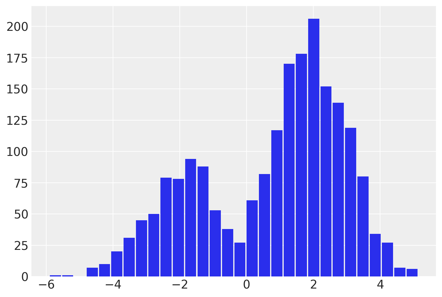
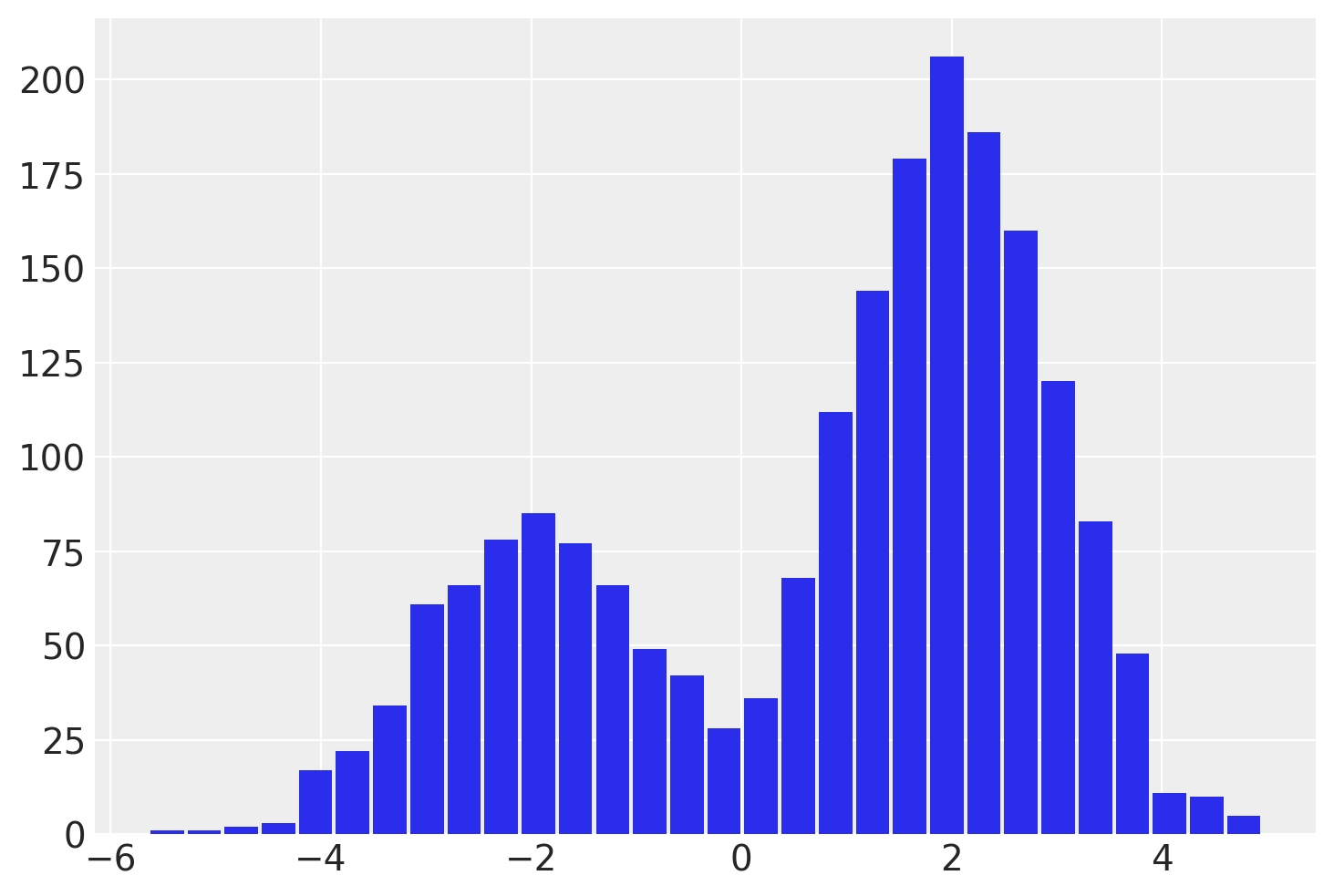
这个 idx 变量让我们在运行NUTS采样器后恢复混合分配变量！我们可以通过从每个样本的相关 idx 中读取混合标签来拆分 y 的样本。

# fmt: off
post = idata.posterior
plt.hist(
    post.where(post.idx == 0).y.values.reshape(-1),
    bins=30,
    rwidth=0.9,
    alpha=0.75,
    label='idx = 0',
)
plt.hist(
    post.where(post.idx == 1).y.values.reshape(-1),
    bins=30,
    rwidth=0.9,
    alpha=0.75,
    label='idx = 1'
)
# fmt: on
plt.legend();

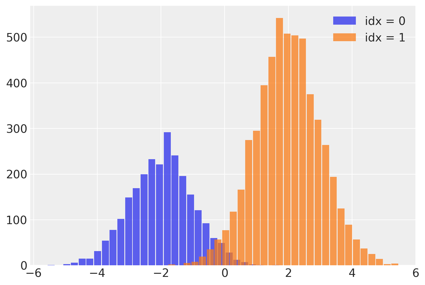
../_images/83e1e4ab30e9d0dd341f132504190325bf794fb5a6a06ea2ef8eee4c4897364d.png

需要注意的一个重要问题是，这个离散变量的有效样本量（ESS）较低，特别是在尾部。这意味着idx可能无法很好地估计，特别是在尾部。如果这一点很重要，我建议使用lp_idx，它是给定每次迭代样本值的idx的对数概率。在下一个示例中将进一步探讨使用lp_idx的好处。

煤矿开采模型#

同样的方法也适用于煤矿开采转折点模型。煤矿开采数据集记录了1851年至1962年间英国煤矿灾难的数量。该时间序列数据集捕捉到了正在引入采矿安全法规的时期，我们尝试使用一个离散的转折点变量来估计这一事件发生的时间。

# fmt: off
disaster_data = pd.Series(
    [4, 5, 4, 0, 1, 4, 3, 4, 0, 6, 3, 3, 4, 0, 2, 6,
    3, 3, 5, 4, 5, 3, 1, 4, 4, 1, 5, 5, 3, 4, 2, 5,
    2, 2, 3, 4, 2, 1, 3, np.nan, 2, 1, 1, 1, 1, 3, 0, 0,
    1, 0, 1, 1, 0, 0, 3, 1, 0, 3, 2, 2, 0, 1, 1, 1,
    0, 1, 0, 1, 0, 0, 0, 2, 1, 0, 0, 0, 1, 1, 0, 2,
    3, 3, 1, np.nan, 2, 1, 1, 1, 1, 2, 4, 2, 0, 0, 1, 4,
    0, 0, 0, 1, 0, 0, 0, 0, 0, 1, 0, 0, 1, 0, 1]
)

# fmt: on
years = np.arange(1851, 1962)

with pmx.MarginalModel() as disaster_model:
    switchpoint = pm.DiscreteUniform("switchpoint", lower=years.min(), upper=years.max())
    early_rate = pm.Exponential("early_rate", 1.0, initval=3)
    late_rate = pm.Exponential("late_rate", 1.0, initval=1)
    rate = pm.math.switch(switchpoint >= years, early_rate, late_rate)
    disasters = pm.Poisson("disasters", rate, observed=disaster_data)

/home/zv/upstream/pymc/pymc/model/core.py:1307: RuntimeWarning: invalid value encountered in cast
  data = convert_observed_data(data).astype(rv_var.dtype)
/home/zv/upstream/pymc/pymc/model/core.py:1321: ImputationWarning: Data in disasters contains missing values and will be automatically imputed from the sampling distribution.
  warnings.warn(impute_message, ImputationWarning)

我们将在边缘化switchpoint变量之前和之后对模型进行采样

with disaster_model:
    before_marg = pm.sample(chains=2, random_seed=rng)

disaster_model.marginalize(["switchpoint"])

with disaster_model:
    after_marg = pm.sample(chains=2, random_seed=rng)

Multiprocess sampling (2 chains in 2 jobs)
CompoundStep
>CompoundStep
>>Metropolis: [switchpoint]
>>Metropolis: [disasters_unobserved]
>NUTS: [early_rate, late_rate]

100.00% [4000/4000 00:07<00:00 Sampling 2 chains, 0 divergences]

Sampling 2 chains for 1_000 tune and 1_000 draw iterations (2_000 + 2_000 draws total) took 8 seconds.
We recommend running at least 4 chains for robust computation of convergence diagnostics
/home/zv/upstream/pymc-experimental/pymc_experimental/model/marginal_model.py:169: UserWarning: There are multiple dependent variables in a FiniteDiscreteMarginalRV. Their joint logp terms will be assigned to the first RV: disasters_unobserved
  warnings.warn(
Multiprocess sampling (2 chains in 2 jobs)
CompoundStep
>NUTS: [early_rate, late_rate]
>Metropolis: [disasters_unobserved]

100.00% [4000/4000 03:11<00:00 Sampling 2 chains, 0 divergences]

Sampling 2 chains for 1_000 tune and 1_000 draw iterations (2_000 + 2_000 draws total) took 191 seconds.
We recommend running at least 4 chains for robust computation of convergence diagnostics

az.summary(before_marg, var_names=["~disasters"], filter_vars="like")

	mean	sd	hdi_3%	hdi_97%	mcse_mean	mcse_sd	ess_bulk	ess_tail	r_hat
switchpoint	1890.224	2.657	1886.000	1896.000	0.192	0.136	201.0	171.0	1.0
early_rate	3.085	0.279	2.598	3.636	0.007	0.005	1493.0	1255.0	1.0
late_rate	0.927	0.114	0.715	1.143	0.003	0.002	1136.0	1317.0	1.0

az.summary(after_marg, var_names=["~disasters"], filter_vars="like")

	mean	sd	hdi_3%	hdi_97%	mcse_mean	mcse_sd	ess_bulk	ess_tail	r_hat
early_rate	3.077	0.289	2.529	3.606	0.007	0.005	1734.0	1150.0	1.0
late_rate	0.932	0.113	0.725	1.150	0.003	0.002	1871.0	1403.0	1.0

如前所述，ESS得到了极大的改善

最后，让我们恢复switchpoint变量

disaster_model.recover_marginals(after_marg);

az.summary(after_marg, var_names=["~disasters", "~lp"], filter_vars="like")

	mean	sd	hdi_3%	hdi_97%	mcse_mean	mcse_sd	ess_bulk	ess_tail	r_hat
early_rate	3.077	0.289	2.529	3.606	0.007	0.005	1734.0	1150.0	1.00
late_rate	0.932	0.113	0.725	1.150	0.003	0.002	1871.0	1403.0	1.00
switchpoint	1889.764	2.458	1886.000	1894.000	0.070	0.050	1190.0	1883.0	1.01

虽然 recover_marginals 能够对被边缘化的离散变量进行采样。每次抽样所关联的概率通常能提供一个更清晰的离散变量估计。特别是对于较低概率值的情况。通过比较采样值的直方图与对数概率图，可以最好地说明这一点。

post = after_marg.posterior.switchpoint.values.reshape(-1)
bins = np.arange(post.min(), post.max())
plt.hist(post, bins, rwidth=0.9);

../_images/35b96b9e05bb5eff4d64a069e5053b3e469a460aa34f42599acdbe76e2972f63.png

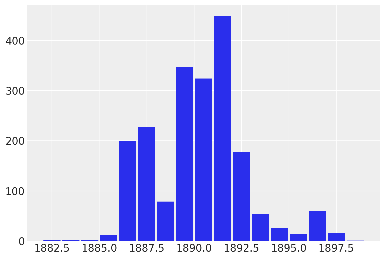
lp_switchpoint = after_marg.posterior.lp_switchpoint.mean(dim=["chain", "draw"])
x_max = years[lp_switchpoint.argmax()]

plt.scatter(years, lp_switchpoint)
plt.axvline(x=x_max, c="orange")
plt.xlabel(r"$\mathrm{year}$")
plt.ylabel(r"$\log p(\mathrm{switchpoint}=\mathrm{year})$");

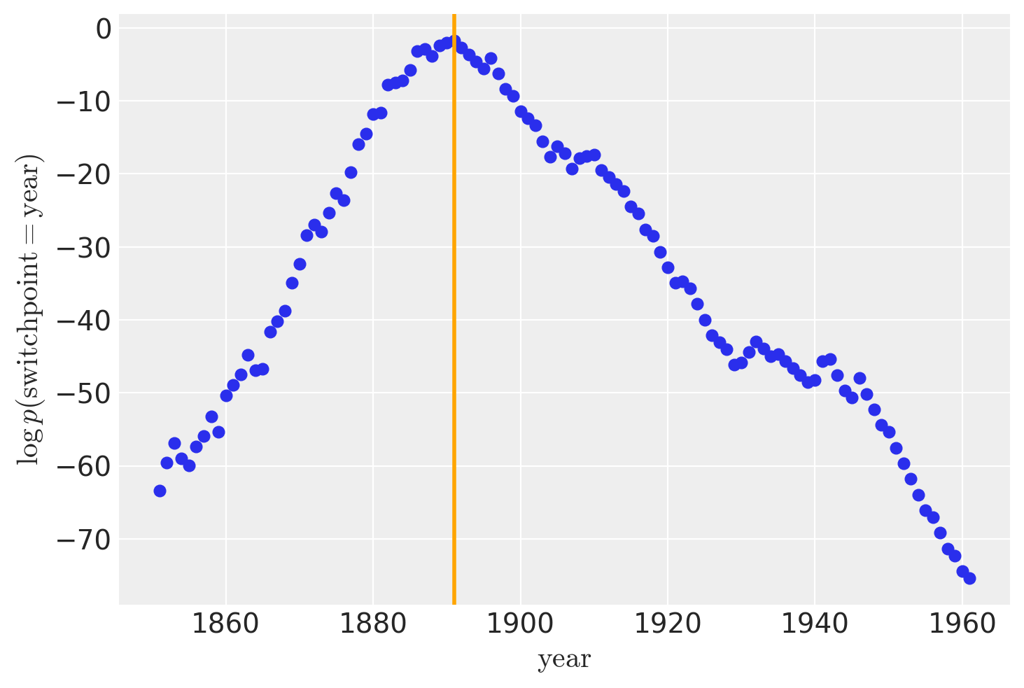
../_images/086b70a2da6286a4f27fda98c2a6750cbc0999785c89b6c31cb34ad269b2dac7.png

通过绘制采样值的直方图而不是直接处理对数概率，我们对底层离散分布的探索变得更加嘈杂和不完整。

作者#

由Rob Zinkov于2024年1月撰写

参考资料#

STAN手册中关于边际化的章节

水印#

%load_ext watermark
%watermark -n -u -v -iv -w -p pytensor,xarray

Last updated: Sat Feb 10 2024

Python implementation: CPython
Python version       : 3.11.6
IPython version      : 8.20.0

pytensor: 2.18.6
xarray  : 2023.11.0

pymc             : 5.11
numpy            : 1.26.3
pytensor         : 2.18.6
pymc_experimental: 0.0.15
arviz            : 0.17.0
pandas           : 2.1.4
matplotlib       : 3.8.2

Watermark: 2.4.3

许可证声明#

本示例库中的所有笔记本均在MIT许可证下提供，该许可证允许修改和重新分发，前提是保留版权和许可证声明。

引用 PyMC 示例#

要引用此笔记本，请使用Zenodo为pymc-examples仓库提供的DOI。

重要

许多笔记本是从其他来源改编的：博客、书籍……在这种情况下，您应该引用原始来源。

同时记得引用代码中使用的相关库。

这是一个BibTeX的引用模板：

@incollection{citekey,
  author    = "<notebook authors, see above>",
  title     = "<notebook title>",
  editor    = "PyMC Team",
  booktitle = "PyMC examples",
  doi       = "10.5281/zenodo.5654871"
}

渲染后可能看起来像：

分类

标签

离散变量的自动边缘化#

高斯混合模型#

煤矿开采模型#

作者#

参考资料#

水印#

许可证声明#

引用 PyMC 示例#