%matplotlib inline
import arviz as az
import matplotlib.pyplot as plt
import numpy as np
import pymc3 as pm
import theano

from pymc3.ode import DifferentialEquation
from scipy.integrate import odeint

plt.style.use("seaborn-darkgrid")
GSoC 2019: pymc3.ode API 的介绍#
常微分方程(ODEs)是建模从工程到生态等学科中系统时间动态的便捷数学框架。尽管大多数分析集中在分岔和固定点的稳定性上,但在实际应用系统中,如群体药代动力学和药效学中,参数和不确定性估计更为重要。
参数估计和不确定性传播都可以通过贝叶斯框架优雅地处理。在这个笔记本中,我展示了如何使用PyMC3的ode子模块来进行微分方程的推断。虽然当前的实现非常灵活且集成良好,但更复杂的模型可能会变得难以估计。一个名为sunode的新包将更快的sundials包集成到PyMC3中,可以在这里找到。
追赶微分方程#
微分方程是关于未知函数的导数与其自身相关的方程。我们通常将微分方程写为
这里,\(\mathbf{y}\) 是未知函数,\(t\) 是时间,\(\mathbf{p}\) 是一个参数向量。函数 \(f\) 可以是标量或向量值。
只有一小部分微分方程具有解析解。对于大多数应用感兴趣的微分方程,必须使用数值方法来获得近似解。
使用微分方程进行贝叶斯推断#
PyMC3 使用哈密尔顿蒙特卡洛(HMC)从后验分布中获取样本。HMC 需要对参数 \(p\) 的 ODE 解的导数。ode 子模块会自动计算适当的导数,因此您不需要手动计算。您只需要做的是
将微分方程写成一个Python函数
在 PyMC3 中编写模型
点击推理按钮 \(^{\text{TM}}\)
让我们通过一个小例子来看看这在实践中是如何完成的。
自由落体的微分方程#
一个质量为 \(m\) 的物体被带到一定高度并允许自由下落,直到它到达地面。描述物体速度随时间变化的微分方程是
物体在向下方向上所受的力是 \(mg\),而物体在相反方向上所受的力(由于空气阻力)与物体当前的运动速度成正比。假设物体从静止状态开始(即物体的初始速度为0)。这可能是也可能不是实际情况。为了展示如何对初始条件进行推断,我首先假设物体从静止状态开始,然后稍后放宽这一假设。
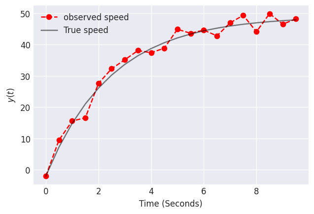
此对象随时间变化的速度数据如下所示。由于我们的测量工具或对象的不规则形状,数据可能存在噪声,这可能导致在自由落体过程中对象的空气动力学性能时好时坏。让我们使用这些数据来估计空气阻力的比例常数。
# For reproducibility
np.random.seed(20394)


def freefall(y, t, p):
    return 2.0 * p[1] - p[0] * y[0]


# Times for observation
times = np.arange(0, 10, 0.5)
gamma, g, y0, sigma = 0.4, 9.8, -2, 2
y = odeint(freefall, t=times, y0=y0, args=tuple([[gamma, g]]))
yobs = np.random.normal(y, 2)

fig, ax = plt.subplots(dpi=120)
plt.plot(times, yobs, label="observed speed", linestyle="dashed", marker="o", color="red")
plt.plot(times, y, label="True speed", color="k", alpha=0.5)
plt.legend()
plt.xlabel("Time (Seconds)")
plt.ylabel(r"$y(t)$")
plt.show()
要使用 pyMC3 指定一个常微分方程,请使用 DifferentialEquation 类。该类接受以下参数:
func: 指定微分方程的函数(即 \(f(\mathbf{y},t,\mathbf{p})\))。times: 数据被观测的时间数组。n_states: \(f(\mathbf{y},t,\mathbf{p})\) 的维度。n_theta: \(\mathbf{p}\) 的维度。t0: 可选的时间,表示初始条件所属的时间点。
参数 func 需要写成好像 y 和 p 是向量的形式。因此,即使你的模型只有一个状态和/或一个参数,你也应该明确地写成 y[0] 和/或 p[0]。
一旦模型被指定,我们可以在我们的pyMC3模型中通过传递参数和初始条件来使用它。DifferentialEquation返回一个扁平化的解,因此你需要在模型中将其重塑为与观测数据相同的形状。
如下所示是一个用于估计上述ODE中\(\gamma\)的模型。
ode_model = DifferentialEquation(func=freefall, times=times, n_states=1, n_theta=2, t0=0)

with pm.Model() as model:
    # Specify prior distributions for some of our model parameters
    sigma = pm.HalfCauchy("sigma", 1)
    gamma = pm.Lognormal("gamma", 0, 1)

    # If we know one of the parameter values, we can simply pass the value.
    ode_solution = ode_model(y0=[0], theta=[gamma, 9.8])
    # The ode_solution has a shape of (n_times, n_states)

    Y = pm.Normal("Y", mu=ode_solution, sigma=sigma, observed=yobs)

    prior = pm.sample_prior_predictive()
    trace = pm.sample(2000, tune=1000, cores=1)
    posterior_predictive = pm.sample_posterior_predictive(trace)

    data = az.from_pymc3(trace=trace, prior=prior, posterior_predictive=posterior_predictive)
Auto-assigning NUTS sampler...
Initializing NUTS using jitter+adapt_diag...
Sequential sampling (2 chains in 1 job)
NUTS: [gamma, sigma]
Sampling 2 chains for 1_000 tune and 2_000 draw iterations (2_000 + 4_000 draws total) took 682 seconds.
az.plot_posterior(data);
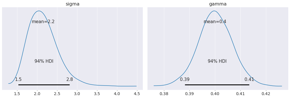
我们对系统中比例常数和噪声的估计与其实际值非常接近!
我们甚至可以通过为重力加速度指定先验来估计它。
with pm.Model() as model2:
    sigma = pm.HalfCauchy("sigma", 1)
    gamma = pm.Lognormal("gamma", 0, 1)
    # A prior on the acceleration due to gravity
    g = pm.Lognormal("g", pm.math.log(10), 2)

    # Notice now I have passed g to the odeparams argument
    ode_solution = ode_model(y0=[0], theta=[gamma, g])

    Y = pm.Normal("Y", mu=ode_solution, sigma=sigma, observed=yobs)

    prior = pm.sample_prior_predictive()
    trace = pm.sample(2000, tune=1000, target_accept=0.9, cores=1)
    posterior_predictive = pm.sample_posterior_predictive(trace)

    data = az.from_pymc3(trace=trace, prior=prior, posterior_predictive=posterior_predictive)
Auto-assigning NUTS sampler...
Initializing NUTS using jitter+adapt_diag...
Sequential sampling (2 chains in 1 job)
NUTS: [g, gamma, sigma]
Sampling 2 chains for 1_000 tune and 2_000 draw iterations (2_000 + 4_000 draws total) took 2595 seconds.
az.plot_posterior(data);
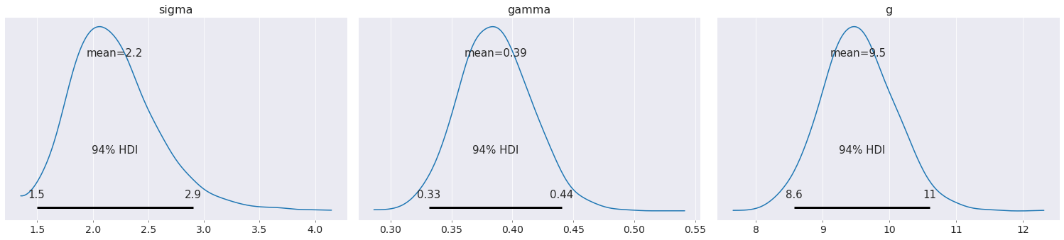
由于重力加速度的不确定性,比例常数的不确定性也增加了。
最后,我们可以对初始条件进行推理。如果这个物体是由飞机带到初始高度的,那么湍流空气可能使飞机上下移动,从而改变了物体的初始速度。
对初始条件进行推理就像为初始条件指定一个先验,然后将初始条件传递给ode_model一样简单。
with pm.Model() as model3:
    sigma = pm.HalfCauchy("sigma", 1)
    gamma = pm.Lognormal("gamma", 0, 1)
    g = pm.Lognormal("g", pm.math.log(10), 2)
    # Initial condition prior.  We think it is at rest, but will allow for perturbations in initial velocity.
    y0 = pm.Normal("y0", 0, 2)

    ode_solution = ode_model(y0=[y0], theta=[gamma, g])

    Y = pm.Normal("Y", mu=ode_solution, sigma=sigma, observed=yobs)

    prior = pm.sample_prior_predictive()
    trace = pm.sample(2000, tune=1000, target_accept=0.9, cores=1)
    posterior_predictive = pm.sample_posterior_predictive(trace)

    data = az.from_pymc3(trace=trace, prior=prior, posterior_predictive=posterior_predictive)
Auto-assigning NUTS sampler...
Initializing NUTS using jitter+adapt_diag...
Sequential sampling (2 chains in 1 job)
NUTS: [y0, g, gamma, sigma]
/env/miniconda3/lib/python3.7/site-packages/scipy/integrate/odepack.py:248: ODEintWarning: Illegal input detected (internal error). Run with full_output = 1 to get quantitative information.
  warnings.warn(warning_msg, ODEintWarning)
Sampling 2 chains for 1_000 tune and 2_000 draw iterations (2_000 + 4_000 draws total) took 3550 seconds.
az.plot_posterior(data, figsize=(13, 3));
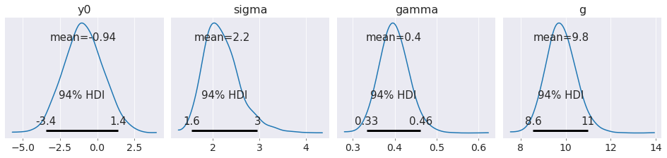
请注意,通过显式建模初始条件,我们得到的由于重力引起的加速度的估计比如果我们坚持物体从静止开始要好得多。
非线性微分方程#
自由落体物体的例子可能不是最合适的,因为那个微分方程可以精确求解。因此,DifferentialEquation 不需要用来解决那个特定的问题。然而,有许多微分方程无法精确求解。这些模型的推理正是 DifferentialEquation 真正发挥作用的地方。
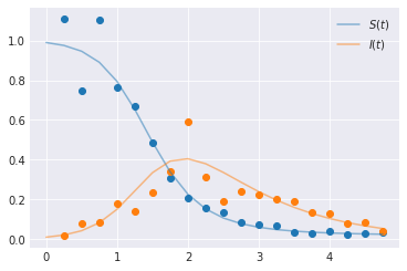
考虑感染的SIR模型。 该模型描述了疾病在均匀混合的封闭人群中传播的时间动态。 人群中的成员被分为三个类别之一:易感者、感染者或康复者。 微分方程是…
在约束条件 \(S(t) + I(t) + R(t) = 1 \, \forall t\) 下。这里,\(\beta\) 是每个易感者和每个感染者的感染率,\(\lambda\) 是恢复率。
如果我们知道 \(S(t)\) 和 \(I(t)\),那么我们可以确定 \(R(t)\),因此我们可以剥离关于 \(R(t)\) 的微分方程,只处理前两个。
在SIR模型中,可以直观地看出\(\beta, \gamma\)和\(\beta/2, \gamma/2\)会产生相同的定性动态,但在非常不同的时间尺度上。为了研究动态的质量,无论时间尺度如何,应用数学家们会无量纲化微分方程。无量纲化是将无量纲变量引入微分方程的过程,以理解系统在等效参数化族下的动态。
为了将这个系统无量纲化,让我们将时间按\(1/\lambda\)进行缩放(我们这样做是因为人们平均感染时间为\(1/\lambda\)个时间单位。这是一个直接的论证,可以证明这一点。更多内容,请参见[1])。设\(t = \tau/\lambda\),其中\(\tau\)是一个无量纲变量。然后…
和
量 \(\beta/\lambda\) 有一个非常特殊的名字。我们称之为 R-Nought (\(\mathcal{R}_0\))。它的解释是,如果我们把一个感染者放入一个易感个体的群体中,我们预计会有 \(\mathcal{R}_0\) 个新的感染。如果 \(\mathcal{R}_0>1\),那么将会发生流行病。如果 \(\mathcal{R}_0\leq1\) 那么就不会有流行病(注意,我们可以通过研究系统雅可比矩阵的特征值来更严格地证明这一点。更多信息,请参见 [2])。
这种无量纲化是重要的,因为它为我们提供了关于参数的信息。如果我们看到已经发生了流行病,那么我们知道 \(\mathcal{R}_0>1\),这意味着 \(\beta> \lambda\)。此外,由于beta的解释,可能很难在 \(\beta\) 上放置先验。但由于 \(1/\lambda\) 有简单的解释,并且由于 \(\mathcal{R}_0>1\),我们可以通过计算 \(\mathcal{R}_0\lambda\) 来获得 \(\beta\)。
旁注:我将选择一个显然违反这些约束的可能性,只是为了说明如何使用DifferentialEquation。实际上,应该选择一个尊重这些约束的可能性。
def SIR(y, t, p):
    ds = -p[0] * y[0] * y[1]
    di = p[0] * y[0] * y[1] - p[1] * y[1]
    return [ds, di]


times = np.arange(0, 5, 0.25)

beta, gamma = 4, 1.0
# Create true curves
y = odeint(SIR, t=times, y0=[0.99, 0.01], args=((beta, gamma),), rtol=1e-8)
# Observational model.  Lognormal likelihood isn't appropriate, but we'll do it anyway
yobs = np.random.lognormal(mean=np.log(y[1::]), sigma=[0.2, 0.3])

plt.plot(times[1::], yobs, marker="o", linestyle="none")
plt.plot(times, y[:, 0], color="C0", alpha=0.5, label=f"$S(t)$")
plt.plot(times, y[:, 1], color="C1", alpha=0.5, label=f"$I(t)$")
plt.legend()
plt.show()
sir_model = DifferentialEquation(
    func=SIR,
    times=np.arange(0.25, 5, 0.25),
    n_states=2,
    n_theta=2,
    t0=0,
)

with pm.Model() as model4:
    sigma = pm.HalfCauchy("sigma", 1, shape=2)

    # R0 is bounded below by 1 because we see an epidemic has occurred
    R0 = pm.Bound(pm.Normal, lower=1)("R0", 2, 3)
    lam = pm.Lognormal("lambda", pm.math.log(2), 2)
    beta = pm.Deterministic("beta", lam * R0)

    sir_curves = sir_model(y0=[0.99, 0.01], theta=[beta, lam])

    Y = pm.Lognormal("Y", mu=pm.math.log(sir_curves), sigma=sigma, observed=yobs)

    trace = pm.sample(2000, tune=1000, target_accept=0.9, cores=1)
    data = az.from_pymc3(trace=trace)
Auto-assigning NUTS sampler...
Initializing NUTS using jitter+adapt_diag...
Sequential sampling (2 chains in 1 job)
NUTS: [lambda, R0, sigma]
Sampling 2 chains for 1_000 tune and 2_000 draw iterations (2_000 + 4_000 draws total) took 5339 seconds.
az.plot_posterior(data, round_to=2, credible_interval=0.95);
/dependencies/arviz/arviz/utils.py:654: UserWarning: Keyword argument credible_interval has been deprecated Please replace with hdi_prob
  ("Keyword argument credible_interval has been deprecated " "Please replace with hdi_prob"),
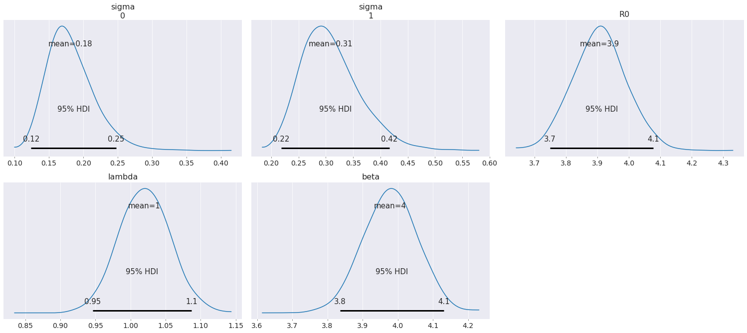
从后验图中可以看出,通过利用关于无量纲参数\(\mathcal{R}_0\)和\(\lambda\)的知识,\(\beta\)得到了很好的估计。
结论与最终想法#
ODEs 是连续时间演化的一个非常好的模型。随着 DifferentialEquation 被添加到 PyMC3 中,我们现在可以使用贝叶斯方法来估计 ODEs 的参数。
DifferentialEquation 相比 Stan 的 integrate_ode_bdf 速度较慢。然而,DifferentialEquation 的易用性将使从业者能够比 Stan(具有陡峭的学习曲线)更快地启动并运行 ODE 的贝叶斯估计。
参考资料#
Earn, D. J. 等人。 《数学流行病学》。 柏林:Springer,2008年。
布里顿, 尼古拉斯 F. 《基础数学生物学》. 斯普林格科学与商业媒体, 2012.
%load_ext watermark
%watermark -n -u -v -iv -w
arviz  0.8.3
theano 1.0.4
pymc3  3.9.0
numpy  1.18.5
last updated: Mon Jun 15 2020

CPython 3.7.7
IPython 7.15.0
watermark 2.0.2