多级重力测量与MLDA#
MLDA采样器#
本笔记本旨在演示Dodwell(2019)提出的多级延迟接受MCMC算法(MLDA),如在PyMC3中实现的那样。如果您是第一次使用MLDA,我们建议首先在同一文件夹中运行MLDA_simple_linear_regression.ipynb笔记本。
在处理计算密集型问题时,MLDA采样器可能比其他MCMC采样器更高效,特别是在我们不仅能够访问所需的(精细)后验分布,还能访问一组精度递减、计算成本递减的近似(粗略)后验分布的情况下。简而言之,我们可以在不同粗细程度上使用多条链,较粗链的样本被用作较细链的提议。研究表明,这可以提高最精细链的有效样本量,从而减少昂贵的精细链似然评估的次数。
笔记本最初定义了描述模型的必要类。这些类使用scipy在前向模型中进行数值求解。然后,它在两个层次(具有不同的粒度)中实例化模型,并生成用于推理的数据。最后,模型类通过Theano Ops传递给两个pymc3模型,并使用三种不同的MCMC方法(包括MLDA)进行推理。最后展示了一些总结结果和比较图,以展示结果。当用户希望使用外部代码来计算其似然(例如,一些快速的PDE求解器)时,使用Theano Ops是常见的,此示例旨在为用户在自己的问题中使用MLDA提供一个起点。
请注意,MLDA采样器是PyMC3中的新功能。用户应对结果持额外批判态度,并在pymc3的github仓库中报告任何问题。
下面显示的笔记本结果是在一台配备2.6 GHz 6核Intel Core i7、32 GB DDR4和macOS 10.15.4的MacBook Pro上生成的。
重力测量#
在本笔记本中,我们解决一个二维重力勘测问题,该问题改编自Hansen(2010)提出的1D问题。
我们的目标是恢复一个已知深度 \(d\) 下方的二维质量分布 \(f(\vec{t})\),从地表测量到的重力场垂直分量 \(g(\vec{s})\) 中恢复。地下质量分布的无限小区域的贡献由以下公式给出:
其中 \(\theta\) 是垂直平面与两点 \(f(\vec{t})\) 和 \(g(\vec{s})\) 之间的直线之间的角度,且 \(r = | \vec{s} - \vec{t} |\) 是两点之间的欧几里得距离。我们利用 \(\sin \theta = \frac{d}{r}\),因此
这得到了积分方程,
其中 \(T = [0,1]^2\) 是函数 \(f(\vec{t})\) 的定义域。这构成了我们的正向模型。
我们使用中点求积法数值求解这个积分。为了简单起见,我们沿每个轴使用相同数量的求积点,因此在离散形式下,我们的正演模型变为
其中 \(\omega_j = \frac{1}{m}\) 是正交权重,\(\hat{f}(\vec{t}_j)\) 是在正交点 \(j = 1, \dots, m\) 处的近似地下质量,而 \(g(\vec{s}_i)\) 是在配点 \(i = 1, \dots, n\) 处的表面测量值。因此,当 \(n > m\) 时,我们处理的是一个超定问题,反之亦然。
这导致了一个线性系统 \(\mathbf{Ax = b}\),其中
在这个特定的问题中,矩阵 \(\mathbf{A}\) 的条件数非常高,导致了一个病态的逆问题,这会带来数值不稳定性以及对于噪声右侧的虚假、通常是振荡的解。这类问题传统上通过某种形式的正则化来解决,但它们可以在贝叶斯逆问题的背景下以自然且优雅的方式处理。
质量分布作为高斯随机过程#
我们将未知的质量分布建模为一个具有Matern 5/2协方差核的高斯随机过程(Rasmussen和Williams,2006):
其中 \(l\) 是协方差长度尺度,\(\sigma^2\) 是方差。
比较#
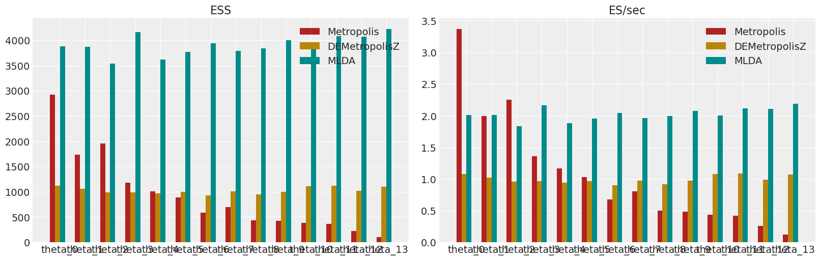
在这个笔记本中,一个简单的MLDA采样器与Metropolis和DEMetropolisZ采样器进行了比较。该示例表明,当以每秒从后验生成的有效样本数来衡量时,MLDA比其他采样器更高效。
参考资料#
Dodwell, Tim & Ketelsen, Chris & Scheichl, Robert & Teckentrup, Aretha. (2019). 多级马尔可夫链蒙特卡洛. SIAM评论. 61. 509-545. https://doi.org/10.1137/19M126966X
佩尔·克里斯蒂安·汉森。《离散逆问题:洞察与算法》。工业与应用数学学会,2010年1月。
卡尔·爱德华·拉斯穆森和克里斯托弗·K·I·威廉姆斯。机器学习的高斯过程。自适应计算和机器学习。2006年。
导入模块#
import os as os
import warnings

os.environ["OPENBLAS_NUM_THREADS"] = "1"  # Set environment variable

import sys as sys
import time as time

import arviz as az
import matplotlib.pyplot as plt
import numpy as np
import pandas as pd
import pymc3 as pm
import theano
import theano.tensor as tt

from numpy.linalg import inv
from scipy.interpolate import RectBivariateSpline
from scipy.linalg import eigh
from scipy.spatial import distance_matrix
warnings.simplefilter(action="ignore", category=FutureWarning)
RANDOM_SEED = 123446
np.random.seed(RANDOM_SEED)
az.style.use("arviz-darkgrid")
# Checking versions
print(f"Theano version: {theano.__version__}")
print(f"PyMC3 version: {pm.__version__}")
Theano version: 1.1.2
PyMC3 version: 3.11.0
定义用于建模高斯随机场的Matern52核#
这是定义模型时所需的实用代码 - 您可以选择忽略它或将它放在外部文件中
class SquaredExponential:
    def __init__(self, coords, mkl, lamb):
        """
        This class sets up a random process
        on a grid and generates
        a realisation of the process, given
        parameters or a random vector.
        """

        # Internalise the grid and set number of vertices.
        self.coords = coords
        self.n_points = self.coords.shape[0]
        self.eigenvalues = None
        self.eigenvectors = None
        self.parameters = None
        self.random_field = None

        # Set some random field parameters.
        self.mkl = mkl
        self.lamb = lamb

        self.assemble_covariance_matrix()

    def assemble_covariance_matrix(self):
        """
        Create a snazzy distance-matrix for rapid
        computation of the covariance matrix.
        """
        dist = distance_matrix(self.coords, self.coords)

        # Compute the covariance between all
        # points in the space.
        self.cov = np.exp(-0.5 * dist**2 / self.lamb**2)

    def plot_covariance_matrix(self):
        """
        Plot the covariance matrix.
        """
        plt.figure(figsize=(10, 8))
        plt.imshow(self.cov, cmap="binary")
        plt.colorbar()
        plt.show()

    def compute_eigenpairs(self):
        """
        Find eigenvalues and eigenvectors using Arnoldi iteration.
        """
        eigvals, eigvecs = eigh(self.cov, eigvals=(self.n_points - self.mkl, self.n_points - 1))

        order = np.flip(np.argsort(eigvals))
        self.eigenvalues = eigvals[order]
        self.eigenvectors = eigvecs[:, order]

    def generate(self, parameters=None):
        """
        Generate a random field, see
        Scarth, C., Adhikari, S., Cabral, P. H.,
        Silva, G. H. C., & Prado, A. P. do. (2019).
        Random field simulation over curved surfaces:
        Applications to computational structural mechanics.
        Computer Methods in Applied Mechanics and Engineering,
        345, 283–301. https://doi.org/10.1016/j.cma.2018.10.026
        """

        if parameters is None:
            self.parameters = np.random.normal(size=self.mkl)
        else:
            self.parameters = np.array(parameters).flatten()

        self.random_field = np.linalg.multi_dot(
            (self.eigenvectors, np.sqrt(np.diag(self.eigenvalues)), self.parameters)
        )

    def plot(self, lognormal=True):
        """
        Plot the random field.
        """

        if lognormal:
            random_field = self.random_field
            contour_levels = np.linspace(min(random_field), max(random_field), 20)
        else:
            random_field = np.exp(self.random_field)
            contour_levels = np.linspace(min(random_field), max(random_field), 20)

        plt.figure(figsize=(12, 10))
        plt.tricontourf(
            self.coords[:, 0],
            self.coords[:, 1],
            random_field,
            levels=contour_levels,
            cmap="plasma",
        )
        plt.colorbar()
        plt.show()


class Matern52(SquaredExponential):
    def assemble_covariance_matrix(self):
        """
        This class inherits from RandomProcess and creates a Matern 5/2 covariance matrix.
        """

        # Compute scaled distances.
        dist = np.sqrt(5) * distance_matrix(self.coords, self.coords) / self.lamb

        # Set up Matern 5/2 covariance matrix.
        self.cov = (1 + dist + dist**2 / 3) * np.exp(-dist)
定义重力模型并生成数据#
由于本案例中使用的模型,这段内容有点长,它包含了类定义以及类对象的实例化和数据生成。
# Set the model parameters.
depth = 0.1
n_quad = 64
n_data = 64
# noise level
noise_level = 0.02
# Set random process parameters.
lamb = 0.1
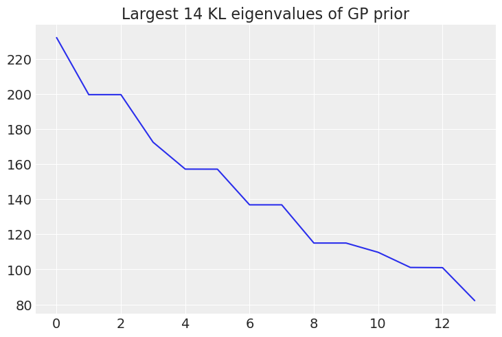
mkl = 14
# Set the quadrature degree for each model level (coarsest first)
n_quadrature = [16, 64]
class Gravity:
"""
Gravity is a class that implements a simple gravity surveying problem,
as described in Hansen, P. C. (2010). Discrete Inverse Problems: Insight and Algorithms.
Society for Industrial and Applied Mathematics.
It uses midpoint quadrature to evaluate a Fredholm integral of the first kind.
"""
def __init__(self, f_function, depth, n_quad, n_data):
# Set the function describing the distribution of subsurface density.
self.f_function = f_function
# Set the depth of the density (distance to the surface measurements).
self.depth = depth
# Set the quadrature degree along one dimension.
self.n_quad = n_quad
# Set the number of data points along one dimension
self.n_data = n_data
# Set the quadrature points.
x = np.linspace(0, 1, self.n_quad + 1)
self.tx = (x[1:] + x[:-1]) / 2
y = np.linspace(0, 1, self.n_quad + 1)
self.ty = (y[1:] + y[:-1]) / 2
TX, TY = np.meshgrid(self.tx, self.ty)
# Set the measurement points.
self.sx = np.linspace(0, 1, self.n_data)
self.sy = np.linspace(0, 1, self.n_data)
SX, SY = np.meshgrid(self.sx, self.sy)
# Create coordinate vectors.
self.T_coords = np.c_[TX.ravel(), TY.ravel(), np.zeros(self.n_quad**2)]
self.S_coords = np.c_[SX.ravel(), SY.ravel(), self.depth * np.ones(self.n_data**2)]
# Set the quadrature weights.
self.w = 1 / self.n_quad**2
# Compute a distance matrix
dist = distance_matrix(self.S_coords, self.T_coords)
# Create the Fremholm kernel.
self.K = self.w * self.depth / dist**3
# Evaluate the density function on the quadrature points.
self.f = self.f_function(TX, TY).flatten()
# Compute the surface density (noiseless measurements)
self.g = np.dot(self.K, self.f)
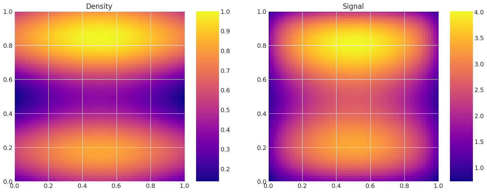
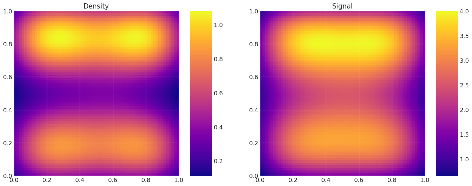
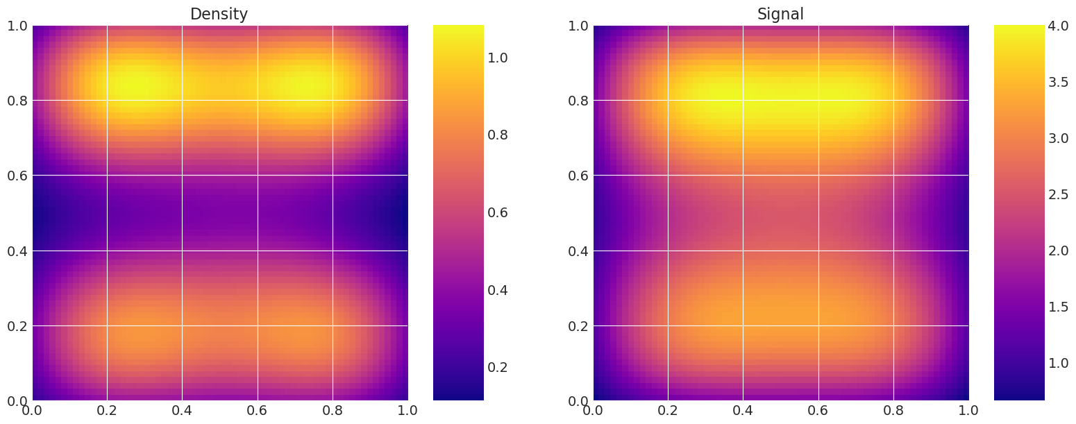
def plot_model(self):
# Plot the density and the signal.
fig, axes = plt.subplots(1, 2, figsize=(16, 6))
axes[0].set_title("Density")
f = axes[0].imshow(
self.f.reshape(self.n_quad, self.n_quad),
extent=(0, 1, 0, 1),
origin="lower",
cmap="plasma",
)
fig.colorbar(f, ax=axes[0])
axes[1].set_title("Signal")
g = axes[1].imshow(
self.g.reshape(self.n_data, self.n_data),
extent=(0, 1, 0, 1),
origin="lower",
cmap="plasma",
)
fig.colorbar(g, ax=axes[1])
plt.show()
def plot_kernel(self):
# Plot the kernel.
plt.figure(figsize=(8, 6))
plt.imshow(self.K, cmap="plasma")
plt.colorbar()
plt.show()
# Initialise a model
model_true = Gravity(f, depth, n_quad, n_data)
model_true.plot_model()
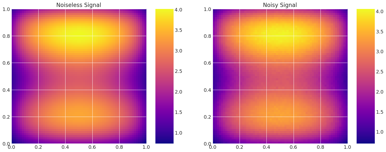
# Add noise to the data.
np.random.seed(123)
noise = np.random.normal(0, noise_level, n_data**2)
data = model_true.g + noise

# Plot the density and the signal.
fig, axes = plt.subplots(1, 2, figsize=(16, 6))
axes[0].set_title("Noiseless Signal")
g = axes[0].imshow(
    model_true.g.reshape(n_data, n_data),
    extent=(0, 1, 0, 1),
    origin="lower",
    cmap="plasma",
)
fig.colorbar(g, ax=axes[0])
axes[1].set_title("Noisy Signal")
d = axes[1].imshow(data.reshape(n_data, n_data), extent=(0, 1, 0, 1), origin="lower", cmap="plasma")
fig.colorbar(d, ax=axes[1])
plt.show()
class Gravity_Forward(Gravity):
    """
    Gravity forward is a class that implements the gravity problem,
    but computation of signal and density is delayed to the "solve"
    method, since it relied on a Gaussian Random Field to model
    the (unknown) density.
    """

    def __init__(self, depth, n_quad, n_data):
        # Set the depth of the density (distance to the surface measurements).
        self.depth = depth

        # Set the quadrature degree along one axis.
        self.n_quad = n_quad

        # Set the number of data points along one axis.
        self.n_data = n_data

        # Set the quadrature points.
        x = np.linspace(0, 1, self.n_quad + 1)
        self.tx = (x[1:] + x[:-1]) / 2
        y = np.linspace(0, 1, self.n_quad + 1)
        self.ty = (y[1:] + y[:-1]) / 2
        TX, TY = np.meshgrid(self.tx, self.ty)

        # Set the measurement points.
        self.sx = np.linspace(0, 1, self.n_data)
        self.sy = np.linspace(0, 1, self.n_data)
        SX, SY = np.meshgrid(self.sx, self.sy)

        # Create coordinate vectors.
        self.T_coords = np.c_[TX.ravel(), TY.ravel(), np.zeros(self.n_quad**2)]
        self.S_coords = np.c_[SX.ravel(), SY.ravel(), self.depth * np.ones(self.n_data**2)]

        # Set the quadrature weights.
        self.w = 1 / self.n_quad**2

        # Compute a distance matrix
        dist = distance_matrix(self.S_coords, self.T_coords)

        # Create the Fremholm kernel.
        self.K = self.w * self.depth / dist**3

    def set_random_process(self, random_process, lamb, mkl):
        # Set the number of KL modes.
        self.mkl = mkl

        # Initialise a random process on the quadrature points.
        # and compute the eigenpairs of the covariance matrix,
        self.random_process = random_process(self.T_coords, self.mkl, lamb)
        self.random_process.compute_eigenpairs()

    def solve(self, parameters):
        # Internalise the Random Field parameters
        self.parameters = parameters

        # Create a realisation of the random process, given the parameters.
        self.random_process.generate(self.parameters)
        mean = 0.0
        stdev = 1.0

        # Set the density.
        self.f = mean + stdev * self.random_process.random_field

        # Compute the signal.
        self.g = np.dot(self.K, self.f)

    def get_data(self):
        # Get the data vector.
        return self.g
# We project the eigenmodes of the fine model to the quadrature points
# of the coarse model using linear interpolation.
def project_eigenmodes(model_coarse, model_fine):
    model_coarse.random_process.eigenvalues = model_fine.random_process.eigenvalues
    for i in range(model_coarse.mkl):
        interpolator = RectBivariateSpline(
            model_fine.tx,
            model_fine.ty,
            model_fine.random_process.eigenvectors[:, i].reshape(
                model_fine.n_quad, model_fine.n_quad
            ),
        )
        model_coarse.random_process.eigenvectors[:, i] = interpolator(
            model_coarse.tx, model_coarse.ty
        ).ravel()
# Initialise the models, according the quadrature degree.
my_models = []
for i, n_quad in enumerate(n_quadrature):
    my_models.append(Gravity_Forward(depth, n_quad, n_data))
    my_models[i].set_random_process(Matern52, lamb, mkl)

# Project the eigenmodes of the fine model to the coarse model.
for m in my_models[:-1]:
    project_eigenmodes(m, my_models[-1])
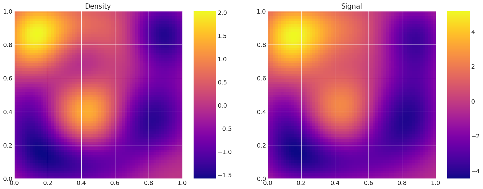
解决并绘制模型以展示粗略/精细差异#
# Plot the same random realisation for each level, and the corresponding signal,
# to validate that the levels are equivalents.
for i, m in enumerate(my_models):
    print(f"Level {i}:")
    np.random.seed(2)
    m.solve(np.random.normal(size=mkl))
    m.plot_model()
Level 0:
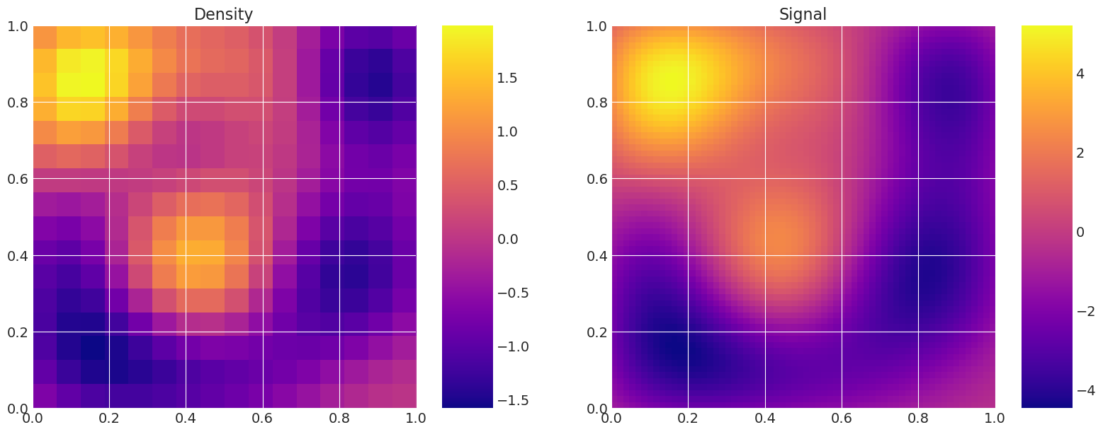
Level 1:
比较粗略和精细模型求解的计算成本#
时间差异越大,MLDA提高效率的潜力就越大
%%timeit
my_models[0].solve(np.random.normal(size=mkl))
259 µs ± 3.7 µs per loop (mean ± std. dev. of 7 runs, 1000 loops each)
%%timeit
my_models[-1].solve(np.random.normal(size=mkl))
5.4 ms ± 122 µs per loop (mean ± std. dev. of 7 runs, 100 loops each)
设置MCMC参数以进行推理#
# Number of draws from the distribution
ndraws = 15000

# Number of burn-in samples
nburn = 10000

# MLDA and Metropolis tuning parameters
tune = True
tune_interval = 100  # Set high to prevent tuning.
discard_tuning = True

# Number of independent chains.
nchains = 3

# Subsampling rate for MLDA
nsub = 5

# Set prior parameters for multivariate Gaussian prior distribution.
mu_prior = np.zeros(mkl)
cov_prior = np.eye(mkl)

# Set the sigma for inference.
sigma = 1.0

# Sampling seed
sampling_seed = RANDOM_SEED
定义一个用于似然的Theano操作#
这将创建将上述模型传递给PyMC3采样器所需的theano操作
def my_loglik(my_model, theta, data, sigma):
    """
    This returns the log-likelihood of my_model given theta,
    datapoints, the observed data and sigma. It uses the
    model_wrapper function to do a model solve.
    """
    my_model.solve(theta)
    output = my_model.get_data()
    return -(0.5 / sigma**2) * np.sum((output - data) ** 2)


class LogLike(tt.Op):
    """
    Theano Op that wraps the log-likelihood computation, necessary to
    pass "black-box" code into pymc3.
    Based on the work in:
    https://docs.pymc.io/notebooks/blackbox_external_likelihood.html
    https://docs.pymc.io/Advanced_usage_of_Theano_in_PyMC3.html
    """

    # Specify what type of object will be passed and returned to the Op when it is
    # called. In our case we will be passing it a vector of values (the parameters
    # that define our model and a model object) and returning a single "scalar"
    # value (the log-likelihood)
    itypes = [tt.dvector]  # expects a vector of parameter values when called
    otypes = [tt.dscalar]  # outputs a single scalar value (the log likelihood)

    def __init__(self, my_model, loglike, data, sigma):
        """
        Initialise the Op with various things that our log-likelihood function
        requires. Below are the things that are needed in this particular
        example.

        Parameters
        ----------
        my_model:
            A Model object (defined in model.py) that contains the parameters
            and functions of out model.
        loglike:
            The log-likelihood function we've defined, in this example it is
            my_loglik.
        data:
            The "observed" data that our log-likelihood function takes in. These
            are the true data generated by the finest model in this example.
        x:
            The dependent variable (aka 'x') that our model requires. This is
            the datapoints in this example.
        sigma:
            The noise standard deviation that our function requires.
        """
        # add inputs as class attributes
        self.my_model = my_model
        self.likelihood = loglike
        self.data = data
        self.sigma = sigma

    def perform(self, node, inputs, outputs):
        # the method that is used when calling the Op
        theta = inputs  # this will contain my variables

        # call the log-likelihood function
        logl = self.likelihood(self.my_model, theta, self.data, self.sigma)

        outputs[0][0] = np.array(logl)  # output the log-likelihood
# create Theano Ops to wrap likelihoods of all model levels and store them in list
logl = []
for i, m_i in enumerate(my_models):
    logl.append(LogLike(m_i, my_loglik, data, sigma))
在 PyMC3 中创建粗略模型#
# Set up models in pymc3 for each level - excluding finest model level
coarse_models = []
for j in range(len(my_models) - 1):
    with pm.Model() as model:
        # Multivariate normal prior.
        theta = pm.MvNormal("theta", mu=mu_prior, cov=cov_prior, shape=mkl)

        # Use the Potential class to evaluate likelihood
        pm.Potential("likelihood", logl[j](theta))

    coarse_models.append(model)
创建精细模型并执行推理#
请注意,我们使用所有三种方法进行采样,并且我们使用MAP作为采样的起点
# Set up finest model and perform inference with PyMC3, using the MLDA algorithm
# and passing the coarse_models list created above.
method_names = []
traces = []
runtimes = []

with pm.Model() as model:
    # Multivariate normal prior.
    theta = pm.MvNormal("theta", mu=mu_prior, cov=cov_prior, shape=mkl)

    # Use the Potential class to evaluate likelihood
    pm.Potential("likelihood", logl[-1](theta))

    # Find the MAP estimate which is used as the starting point for sampling
    MAP = pm.find_MAP()

    # Initialise a Metropolis, DEMetropolisZ and MLDA step method objects (passing the subsampling rate and
    # coarse models list for the latter)
    step_metropolis = pm.Metropolis(tune=tune, tune_interval=tune_interval)
    step_demetropolisz = pm.DEMetropolisZ(tune_interval=tune_interval)
    step_mlda = pm.MLDA(
        coarse_models=coarse_models, subsampling_rates=nsub, base_tune_interval=tune_interval
    )

    # Inference!
    # Metropolis
    t_start = time.time()
    method_names.append("Metropolis")
    traces.append(
        pm.sample(
            draws=ndraws,
            step=step_metropolis,
            chains=nchains,
            tune=nburn,
            discard_tuned_samples=discard_tuning,
            random_seed=sampling_seed,
            start=MAP,
            cores=1,
            mp_ctx="forkserver",
        )
    )
    runtimes.append(time.time() - t_start)

    # DEMetropolisZ
    t_start = time.time()
    method_names.append("DEMetropolisZ")
    traces.append(
        pm.sample(
            draws=ndraws,
            step=step_demetropolisz,
            chains=nchains,
            tune=nburn,
            discard_tuned_samples=discard_tuning,
            random_seed=sampling_seed,
            start=MAP,
            cores=1,
            mp_ctx="forkserver",
        )
    )
    runtimes.append(time.time() - t_start)

    # MLDA
    t_start = time.time()
    method_names.append("MLDA")
    traces.append(
        pm.sample(
            draws=ndraws,
            step=step_mlda,
            chains=nchains,
            tune=nburn,
            discard_tuned_samples=discard_tuning,
            random_seed=sampling_seed,
            start=MAP,
            cores=1,
            mp_ctx="forkserver",
        )
    )
    runtimes.append(time.time() - t_start)
Warning: gradient not available.(E.g. vars contains discrete variables). MAP estimates may not be accurate for the default parameters. Defaulting to non-gradient minimization 'Powell'.
/Users/CloudChaoszero/Documents/Projects-Dev/pymc3/pymc3/step_methods/mlda.py:386: UserWarning: The MLDA implementation in PyMC3 is still immature. You should be particularly critical of its results.
  warnings.warn(
Sequential sampling (3 chains in 1 job)
Metropolis: [theta]
Sampling 3 chains for 10_000 tune and 15_000 draw iterations (30_000 + 45_000 draws total) took 866 seconds.
The rhat statistic is larger than 1.05 for some parameters. This indicates slight problems during sampling.
The estimated number of effective samples is smaller than 200 for some parameters.
Sequential sampling (3 chains in 1 job)
DEMetropolisZ: [theta]
Sampling 3 chains for 10_000 tune and 15_000 draw iterations (30_000 + 45_000 draws total) took 1029 seconds.
The number of effective samples is smaller than 10% for some parameters.
Sequential sampling (3 chains in 1 job)
MLDA: [theta]
The number of effective samples is smaller than 10% for some parameters.
获取后采样统计信息和诊断#
打印 MAP 估计值和 pymc3 采样摘要#
with model:
    print(
        f"\nDetailed summaries and plots:\nMAP estimate: {MAP['theta']}. Not used as starting point."
    )
    for i, trace in enumerate(traces):
        print(f"\n{method_names[i]} Sampler:\n")
        display(az.summary(trace))
Detailed summaries and plots:
MAP estimate: [ 2.27538512e+00  1.88388201e-01 -2.23633947e-01  3.35677618e-04
  1.47801781e+00 -8.33319176e-01  7.28992752e-02 -7.31399445e-02
 -1.01774451e-01 -1.24098721e-01  4.56230029e-01 -1.30949052e-04
  1.37797972e-03  4.16419123e-02]. Not used as starting point.

Metropolis Sampler:
| mean | sd | hdi_3% | hdi_97% | mcse_mean | mcse_sd | ess_mean | ess_sd | ess_bulk | ess_tail | r_hat | |
|---|---|---|---|---|---|---|---|---|---|---|---|
| theta[0] | 2.276 | 0.015 | 2.248 | 2.303 | 0.000 | 0.000 | 2925.0 | 2925.0 | 2925.0 | 4999.0 | 1.00 |
| theta[1] | 0.189 | 0.020 | 0.150 | 0.226 | 0.000 | 0.000 | 1729.0 | 1729.0 | 1730.0 | 3492.0 | 1.00 |
| theta[2] | -0.224 | 0.020 | -0.264 | -0.187 | 0.000 | 0.000 | 1952.0 | 1952.0 | 1953.0 | 3505.0 | 1.00 |
| theta[3] | 0.000 | 0.026 | -0.046 | 0.052 | 0.001 | 0.001 | 1177.0 | 1177.0 | 1179.0 | 1925.0 | 1.00 |
| theta[4] | 1.478 | 0.029 | 1.421 | 1.531 | 0.001 | 0.001 | 1013.0 | 1012.0 | 1013.0 | 2008.0 | 1.00 |
| theta[5] | -0.833 | 0.028 | -0.885 | -0.780 | 0.001 | 0.001 | 889.0 | 889.0 | 892.0 | 1601.0 | 1.01 |
| theta[6] | 0.070 | 0.037 | -0.004 | 0.137 | 0.002 | 0.001 | 586.0 | 586.0 | 587.0 | 1191.0 | 1.00 |
| theta[7] | -0.073 | 0.036 | -0.142 | -0.007 | 0.001 | 0.001 | 695.0 | 695.0 | 695.0 | 1222.0 | 1.00 |
| theta[8] | -0.100 | 0.044 | -0.180 | -0.016 | 0.002 | 0.002 | 429.0 | 429.0 | 431.0 | 1038.0 | 1.01 |
| theta[9] | -0.118 | 0.046 | -0.206 | -0.030 | 0.002 | 0.002 | 421.0 | 421.0 | 421.0 | 832.0 | 1.01 |
| theta[10] | 0.456 | 0.048 | 0.366 | 0.546 | 0.002 | 0.002 | 379.0 | 377.0 | 379.0 | 838.0 | 1.01 |
| theta[11] | -0.001 | 0.053 | -0.096 | 0.104 | 0.003 | 0.002 | 363.0 | 363.0 | 363.0 | 671.0 | 1.01 |
| theta[12] | -0.001 | 0.058 | -0.109 | 0.106 | 0.004 | 0.003 | 224.0 | 224.0 | 225.0 | 552.0 | 1.00 |
| theta[13] | 0.040 | 0.071 | -0.088 | 0.173 | 0.007 | 0.005 | 111.0 | 111.0 | 106.0 | 348.0 | 1.06 |
DEMetropolisZ Sampler:
| mean | sd | hdi_3% | hdi_97% | mcse_mean | mcse_sd | ess_mean | ess_sd | ess_bulk | ess_tail | r_hat | |
|---|---|---|---|---|---|---|---|---|---|---|---|
| theta[0] | 2.275 | 0.015 | 2.247 | 2.302 | 0.000 | 0.000 | 1114.0 | 1114.0 | 1115.0 | 2017.0 | 1.0 |
| theta[1] | 0.188 | 0.020 | 0.150 | 0.226 | 0.001 | 0.000 | 1053.0 | 1046.0 | 1056.0 | 1822.0 | 1.0 |
| theta[2] | -0.223 | 0.020 | -0.259 | -0.183 | 0.001 | 0.000 | 986.0 | 977.0 | 991.0 | 1524.0 | 1.0 |
| theta[3] | 0.000 | 0.025 | -0.049 | 0.047 | 0.001 | 0.001 | 990.0 | 990.0 | 991.0 | 1826.0 | 1.0 |
| theta[4] | 1.478 | 0.030 | 1.418 | 1.533 | 0.001 | 0.001 | 969.0 | 969.0 | 972.0 | 1961.0 | 1.0 |
| theta[5] | -0.833 | 0.030 | -0.889 | -0.777 | 0.001 | 0.001 | 994.0 | 994.0 | 995.0 | 2251.0 | 1.0 |
| theta[6] | 0.072 | 0.036 | 0.008 | 0.140 | 0.001 | 0.001 | 928.0 | 928.0 | 930.0 | 2121.0 | 1.0 |
| theta[7] | -0.073 | 0.036 | -0.136 | 0.000 | 0.001 | 0.001 | 1001.0 | 1001.0 | 1005.0 | 1682.0 | 1.0 |
| theta[8] | -0.103 | 0.046 | -0.189 | -0.013 | 0.002 | 0.001 | 945.0 | 945.0 | 947.0 | 1927.0 | 1.0 |
| theta[9] | -0.124 | 0.045 | -0.207 | -0.039 | 0.001 | 0.001 | 1002.0 | 1002.0 | 1002.0 | 2001.0 | 1.0 |
| theta[10] | 0.458 | 0.050 | 0.368 | 0.553 | 0.001 | 0.001 | 1109.0 | 1109.0 | 1110.0 | 1778.0 | 1.0 |
| theta[11] | 0.003 | 0.053 | -0.099 | 0.098 | 0.002 | 0.001 | 1122.0 | 1122.0 | 1123.0 | 1952.0 | 1.0 |
| theta[12] | 0.001 | 0.054 | -0.099 | 0.104 | 0.002 | 0.001 | 1014.0 | 1014.0 | 1016.0 | 1691.0 | 1.0 |
| theta[13] | 0.040 | 0.071 | -0.093 | 0.171 | 0.002 | 0.002 | 1100.0 | 1100.0 | 1100.0 | 2144.0 | 1.0 |
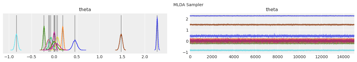
MLDA Sampler:
| mean | sd | hdi_3% | hdi_97% | mcse_mean | mcse_sd | ess_mean | ess_sd | ess_bulk | ess_tail | r_hat | |
|---|---|---|---|---|---|---|---|---|---|---|---|
| theta[0] | 2.275 | 0.015 | 2.247 | 2.303 | 0.000 | 0.000 | 3883.0 | 3882.0 | 3881.0 | 7213.0 | 1.0 |
| theta[1] | 0.189 | 0.020 | 0.151 | 0.227 | 0.000 | 0.000 | 3870.0 | 3870.0 | 3871.0 | 7048.0 | 1.0 |
| theta[2] | -0.224 | 0.020 | -0.262 | -0.185 | 0.000 | 0.000 | 3535.0 | 3530.0 | 3537.0 | 7626.0 | 1.0 |
| theta[3] | 0.001 | 0.026 | -0.049 | 0.049 | 0.000 | 0.000 | 4165.0 | 4165.0 | 4164.0 | 8082.0 | 1.0 |
| theta[4] | 1.478 | 0.029 | 1.423 | 1.534 | 0.000 | 0.000 | 3626.0 | 3620.0 | 3621.0 | 6677.0 | 1.0 |
| theta[5] | -0.834 | 0.030 | -0.890 | -0.778 | 0.000 | 0.000 | 3770.0 | 3767.0 | 3769.0 | 8090.0 | 1.0 |
| theta[6] | 0.073 | 0.037 | 0.002 | 0.141 | 0.001 | 0.000 | 3941.0 | 3941.0 | 3942.0 | 7531.0 | 1.0 |
| theta[7] | -0.073 | 0.037 | -0.142 | -0.003 | 0.001 | 0.000 | 3786.0 | 3786.0 | 3788.0 | 7152.0 | 1.0 |
| theta[8] | -0.103 | 0.046 | -0.190 | -0.017 | 0.001 | 0.001 | 3837.0 | 3837.0 | 3838.0 | 7555.0 | 1.0 |
| theta[9] | -0.124 | 0.046 | -0.208 | -0.035 | 0.001 | 0.001 | 3996.0 | 3996.0 | 4000.0 | 7458.0 | 1.0 |
| theta[10] | 0.457 | 0.049 | 0.364 | 0.550 | 0.001 | 0.001 | 3854.0 | 3823.0 | 3859.0 | 7195.0 | 1.0 |
| theta[11] | 0.000 | 0.055 | -0.101 | 0.104 | 0.001 | 0.001 | 4079.0 | 4079.0 | 4076.0 | 7430.0 | 1.0 |
| theta[12] | 0.000 | 0.056 | -0.103 | 0.105 | 0.001 | 0.001 | 4068.0 | 4068.0 | 4069.0 | 7309.0 | 1.0 |
| theta[13] | 0.043 | 0.071 | -0.096 | 0.173 | 0.001 | 0.001 | 4223.0 | 4223.0 | 4224.0 | 6875.0 | 1.0 |
显示所有采样器的ESS和ESS/秒#
acc = []
ess = []
ess_n = []
performances = []

# Get some more statistics.
with model:
    for i, trace in enumerate(traces):
        acc.append(trace.get_sampler_stats("accepted").mean())
        ess.append(np.array(az.ess(trace).to_array()))
        ess_n.append(ess[i] / len(trace) / trace.nchains)
        performances.append(ess[i] / runtimes[i])
        print(
            f"\n{method_names[i]} Sampler: {len(trace)} drawn samples in each of "
            f"{trace.nchains} chains."
            f"\nRuntime: {runtimes[i]} seconds"
            f"\nAcceptance rate: {acc[i]}"
            f"\nESS list: {np.round(ess[i][0], 3)}"
            f"\nNormalised ESS list: {np.round(ess_n[i][0], 3)}"
            f"\nESS/sec: {np.round(performances[i][0], 3)}"
        )

    # Plot the effective sample size (ESS) and relative ESS (ES/sec) of each of the sampling strategies.
    colors = ["firebrick", "darkgoldenrod", "darkcyan", "olivedrab"]

    fig, axes = plt.subplots(1, 2, figsize=(16, 5))

    axes[0].set_title("ESS")
    for i, e in enumerate(ess):
        axes[0].bar(
            [j + i * 0.2 for j in range(mkl)],
            e.ravel(),
            width=0.2,
            color=colors[i],
            label=method_names[i],
        )
    axes[0].set_xticks([i + 0.3 for i in range(mkl)])
    axes[0].set_xticklabels([f"theta_{i}" for i in range(mkl)])
    axes[0].legend()

    axes[1].set_title("ES/sec")
    for i, p in enumerate(performances):
        axes[1].bar(
            [j + i * 0.2 for j in range(mkl)],
            p.ravel(),
            width=0.2,
            color=colors[i],
            label=method_names[i],
        )
    axes[1].set_xticks([i + 0.3 for i in range(mkl)])
    axes[1].set_xticklabels([f"theta_{i}" for i in range(mkl)])
    axes[1].legend()
    plt.show()
Metropolis Sampler: 15000 drawn samples in each of 3 chains.
Runtime: 867.003182888031 seconds
Acceptance rate: 0.3532222222222222
ESS list: [2925.385 1729.714 1952.545 1178.667 1013.358  892.182  587.109  694.838
  431.325  421.477  379.216  363.206  224.562  106.035]
Normalised ESS list: [0.065 0.038 0.043 0.026 0.023 0.02  0.013 0.015 0.01  0.009 0.008 0.008
 0.005 0.002]
ESS/sec: [3.374 1.995 2.252 1.359 1.169 1.029 0.677 0.801 0.497 0.486 0.437 0.419
 0.259 0.122]

DEMetropolisZ Sampler: 15000 drawn samples in each of 3 chains.
Runtime: 1030.1275491714478 seconds
Acceptance rate: 0.27555555555555555
ESS list: [1114.831 1056.146  991.239  991.406  972.288  994.705  929.785 1004.907
  947.364 1002.483 1110.082 1122.778 1016.407 1099.898]
Normalised ESS list: [0.025 0.023 0.022 0.022 0.022 0.022 0.021 0.022 0.021 0.022 0.025 0.025
 0.023 0.024]
ESS/sec: [1.082 1.025 0.962 0.962 0.944 0.966 0.903 0.976 0.92  0.973 1.078 1.09
 0.987 1.068]

MLDA Sampler: 15000 drawn samples in each of 3 chains.
Runtime: 1926.6128001213074 seconds
Acceptance rate: 0.7311777777777778
ESS list: [3880.842 3871.24  3536.667 4163.642 3620.606 3768.901 3941.67  3788.182
 3837.754 3999.578 3859.423 4075.985 4069.313 4224.038]
Normalised ESS list: [0.086 0.086 0.079 0.093 0.08  0.084 0.088 0.084 0.085 0.089 0.086 0.091
 0.09  0.094]
ESS/sec: [2.014 2.009 1.836 2.161 1.879 1.956 2.046 1.966 1.992 2.076 2.003 2.116
 2.112 2.192]
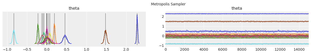
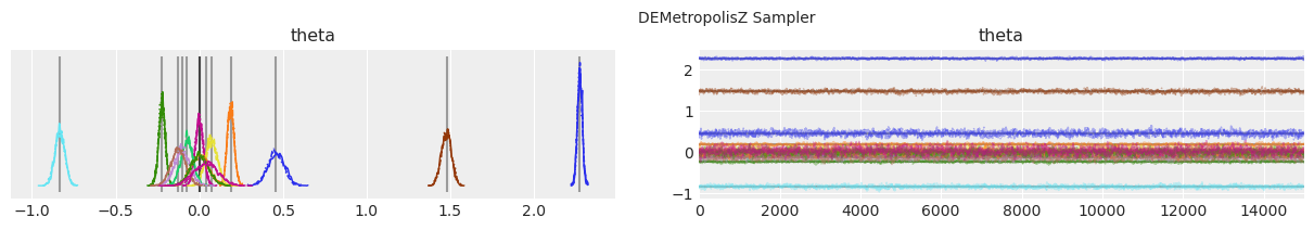
绘制分布和轨迹。#
垂直的灰色线条表示每个参数的最大后验估计值。
with model:
    lines = (("theta", {}, MAP["theta"].tolist()),)
    for i, trace in enumerate(traces):
        az.plot_trace(trace, lines=lines)

        # Ugly hack to get some titles in.
        x_offset = -0.1 * ndraws
        y_offset = trace.get_values("theta").max() + 0.25 * (
            trace.get_values("theta").max() - trace.get_values("theta").min()
        )
        plt.text(x_offset, y_offset, "{} Sampler".format(method_names[i]))
绘制真实和恢复的密度#
这对于验证很有用,即比较真实模型密度和信号与采样器估计的密度和信号。
print("True Model")
model_true.plot_model()
with model:
    print("MAP estimate:")
    my_models[-1].solve(MAP["theta"])
    my_models[-1].plot_model()
    for i, t in enumerate(traces):
        print(f"Recovered by: {method_names[i]}")
        my_models[-1].solve(az.summary(t)["mean"].values)
        my_models[-1].plot_model()
True Model
MAP estimate:
Recovered by: Metropolis

Recovered by: DEMetropolisZ

Recovered by: MLDA
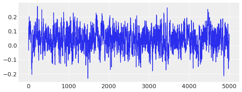
# Show trace of lowest energy mode for Metropolis sampler
plt.figure(figsize=(8, 3))
plt.plot(traces[0]["theta"][:5000, -1])
plt.show()
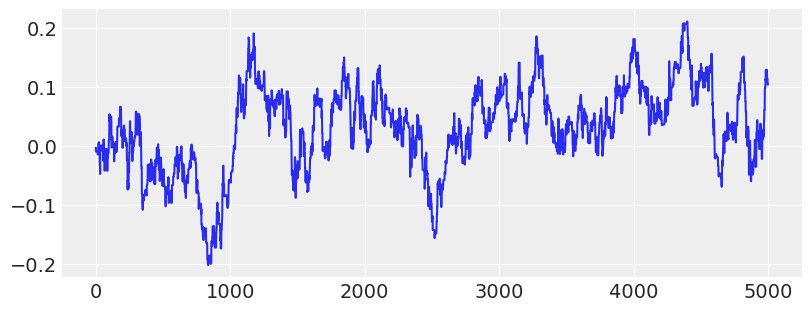
# Show trace of lowest energy mode for MLDA sampler
plt.figure(figsize=(8, 3))
plt.plot(traces[2]["theta"][:5000:, -1])
plt.show()
%load_ext watermark
%watermark -n -u -v -iv -w
Last updated: Sat Feb 06 2021

Python implementation: CPython
Python version       : 3.8.6
IPython version      : 7.20.0

numpy     : 1.20.0
pandas    : 1.2.1
pymc3     : 3.11.0
sys       : 3.8.6 | packaged by conda-forge | (default, Jan 25 2021, 23:22:12)
[Clang 11.0.1 ]
theano    : 1.1.2
matplotlib: None
arviz     : 0.11.0

Watermark: 2.1.0