MLDA采样器#
本笔记本是了解在 PyMC 中实现的 [1] 提出的多级延迟接受 MCMC 算法 (MLDA) 基本用法的良好起点。
它使用了一个简单的线性回归模型(和一个玩具粗略模型作为对照)来展示使用MLDA时的基本工作流程。该模型类似于GLM: 线性回归中使用的模型。
MLDA采样器旨在处理计算密集型问题,我们不仅可以访问所需的(精细)后验分布,还可以访问一组精度递减、计算成本递减的近似(粗略)后验分布(我们至少需要其中一个)。其主要思想是使用较粗链的样本作为较细链的提议。一个粗链运行固定次数的迭代,最后一个样本被用作较细链的提议。这已被证明可以提高最精细链的有效样本量,并且这使我们能够减少昂贵的精细链似然评估的次数。
PyMC 实现支持:
任意数量的层级
两种底层采样器(Metropolis, DEMetropolisZ)
底层采样器的各种调优参数
每个级别的单独子采样率
在底层Metropolis中选择阻塞采样和复合采样的选项。
一种自适应误差模型,用于校正粗略模型和精细模型之间的偏差
一种方差减少技术,利用所有链的样本减少感兴趣估计量的方差。
关于MLDA采样器的更多详细信息以及如何使用和参数化它,用户可以参考代码中的文档字符串和其他处理更复杂问题设置和更高级MLDA功能的示例笔记本。
请注意,MLDA采样器是PyMC中的新功能。用户应对结果持额外批判态度,并在PyMC的GitHub仓库中报告任何问题。
[1] Dodwell, Tim & Ketelsen, Chris & Scheichl, Robert & Teckentrup, Aretha. (2019). 多级马尔可夫链蒙特卡洛. SIAM评论. 61. 509-545. https://doi.org/10.1137/19M126966X
工作流程#
MLDA 的使用方式与 PyMC 中的大多数步骤方法类似。它有一个特殊的要求,即用户需要提供至少一个粗略模型以使其正常工作。
使用MLDA的基本流程包括四个步骤,我们在这里通过一个简单的线性回归模型和一个玩具粗模型来演示。
步骤 1:生成一些数据#
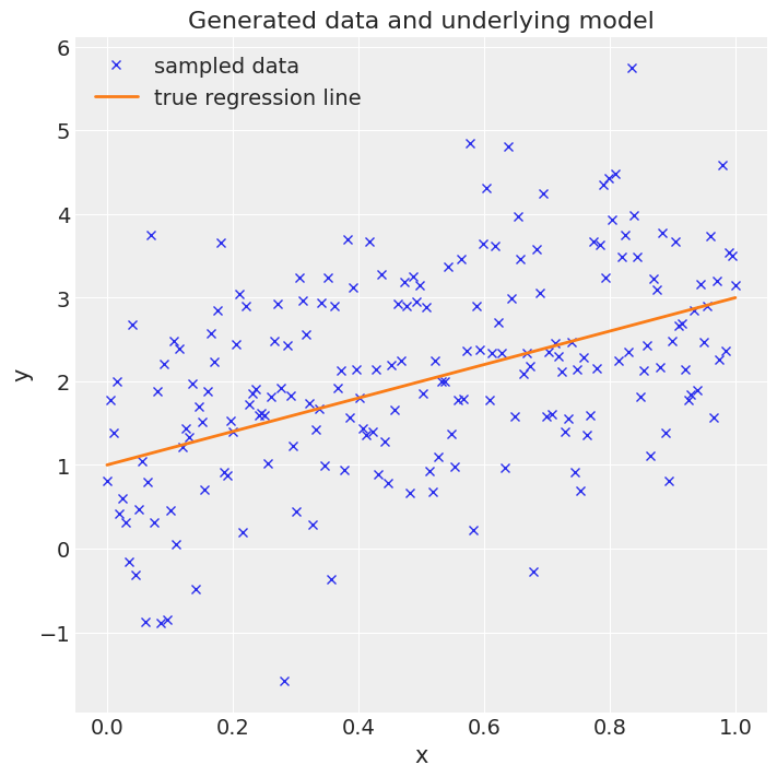
在这里,我们生成一个包含200个等间距点在0.0和1.0之间的向量x。然后我们将这些点投影到截距为1.0、斜率为2.0的直线上,并添加一些随机噪声,得到向量y。目标是根据x和y推断出截距和斜率,即一个非常简单的线性回归问题。
# Import libraries
import time as time
import warnings

import arviz as az
import matplotlib.pyplot as plt
import numpy as np
import pymc as pm
az.style.use("arviz-darkgrid")
warnings.filterwarnings("ignore")
# Generate data
RANDOM_SEED = 915623497
np.random.seed(RANDOM_SEED)

true_intercept = 1
true_slope = 2
sigma = 1

size = 200
x = np.linspace(0, 1, size)
y = true_intercept + true_slope * x + np.random.normal(0, sigma**2, size)
# Plot the data
fig = plt.figure(figsize=(7, 7))
ax = fig.add_subplot(111, xlabel="x", ylabel="y", title="Generated data and underlying model")
ax.plot(x, y, "x", label="sampled data")
ax.plot(x, true_intercept + true_slope * x, label="true regression line", lw=2.0)
plt.legend(loc=0);
步骤 2:定义精细模型#
在这一步中,我们使用PyMC模型定义语言来定义先验和似然。我们为截距和斜率选择无信息的正态先验,并选择正态似然,其中我们输入x和y。
步骤 3:定义一个粗略模型#
在这里,我们定义了一个简单的粗模型,通过在似然中使用比精细模型更少的数据来引入粗糙度,即我们只使用原始数据集中每隔一个的数据点。
# Thinning the data set
x_coarse = x[::2]
y_coarse = y[::2]
步骤4:使用MLDA从后验分布中抽取MCMC样本#
我们将coarse_model传递给MLDA实例,并将subsampling_rate设置为10。子采样率是从粗链中抽取的样本数量,用于为细链构建建议。在这种情况下,MLDA在粗链中抽取10个样本,并使用最后一个样本作为细链的建议。该建议被细链接受或拒绝,然后控制返回到粗链,粗链生成另外10个样本,依此类推。请注意,pm.MLDA还有许多其他调优参数,可以在文档中找到。
接下来,我们使用通用的 pm.sample 方法,将 MLDA 实例传递给它。这将运行 MLDA 并返回一个 trace,其中包含所有 MCMC 样本和各种副产品。在这里,我们还运行了标准 Metropolis 和 DEMetropolisZ 采样器以进行比较,它们返回单独的 traces。我们记录运行时间以便稍后比较。
最后,PyMC 提供了各种函数来可视化轨迹并打印汇总统计信息(以下显示了其中的两个)。
with fine_model:
    # Initialise step methods
    step = pm.MLDA(coarse_models=[coarse_model], subsampling_rates=[10])
    step_2 = pm.Metropolis()
    step_3 = pm.DEMetropolisZ()

    # Sample using MLDA
    t_start = time.time()
    trace = pm.sample(draws=6000, chains=4, tune=2000, step=step, random_seed=RANDOM_SEED)
    runtime = time.time() - t_start

    # Sample using Metropolis
    t_start = time.time()
    trace_2 = pm.sample(draws=6000, chains=4, tune=2000, step=step_2, random_seed=RANDOM_SEED)
    runtime_2 = time.time() - t_start

    # Sample using DEMetropolisZ
    t_start = time.time()
    trace_3 = pm.sample(draws=6000, chains=4, tune=2000, step=step_3, random_seed=RANDOM_SEED)
    runtime_3 = time.time() - t_start
Multiprocess sampling (4 chains in 4 jobs)
MLDA: [slope, intercept]
Sampling 4 chains for 2_000 tune and 6_000 draw iterations (8_000 + 24_000 draws total) took 243 seconds.
Multiprocess sampling (4 chains in 4 jobs)
CompoundStep
>Metropolis: [intercept]
>Metropolis: [slope]
Sampling 4 chains for 2_000 tune and 6_000 draw iterations (8_000 + 24_000 draws total) took 33 seconds.
The number of effective samples is smaller than 10% for some parameters.
Multiprocess sampling (4 chains in 4 jobs)
DEMetropolisZ: [slope, intercept]
Sampling 4 chains for 2_000 tune and 6_000 draw iterations (8_000 + 24_000 draws total) took 32 seconds.
The number of effective samples is smaller than 25% for some parameters.
# Trace plots
az.plot_trace(trace)
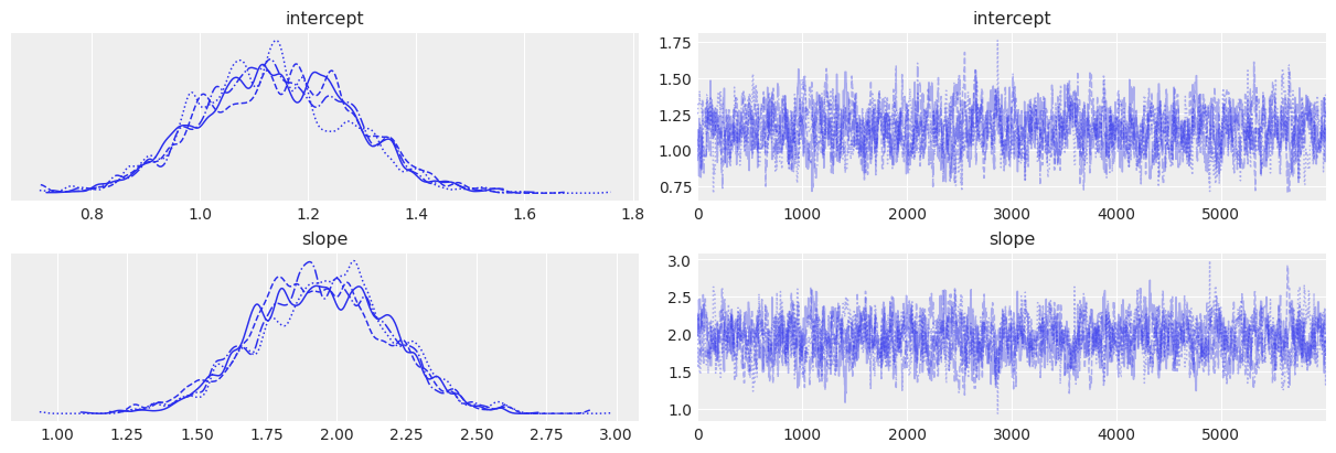
az.plot_trace(trace_2)
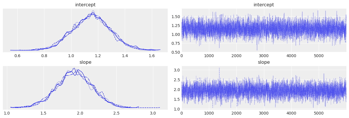
az.plot_trace(trace_3)
array([[<AxesSubplot:title={'center':'intercept'}>,
        <AxesSubplot:title={'center':'intercept'}>],
       [<AxesSubplot:title={'center':'slope'}>,
        <AxesSubplot:title={'center':'slope'}>]], dtype=object)
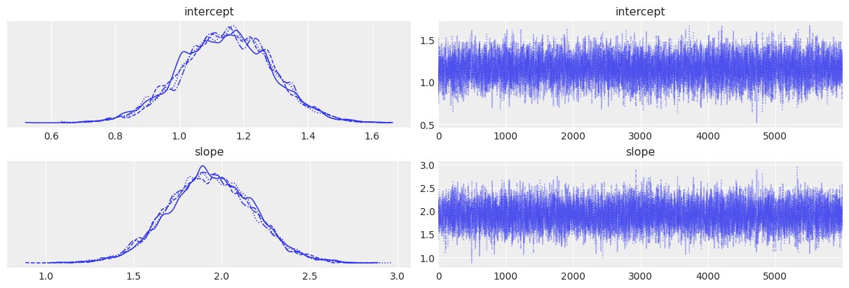
# Summary statistics for MLDA
az.summary(trace)
| mean | sd | hdi_3% | hdi_97% | mcse_mean | mcse_sd | ess_bulk | ess_tail | r_hat | |
|---|---|---|---|---|---|---|---|---|---|
| intercept | 1.146 | 0.141 | 0.875 | 1.406 | 0.002 | 0.001 | 6983.0 | 7758.0 | 1.0 |
| slope | 1.934 | 0.243 | 1.464 | 2.370 | 0.003 | 0.002 | 7289.0 | 7936.0 | 1.0 |
# Summary statistics for Metropolis
az.summary(trace_2)
| mean | sd | hdi_3% | hdi_97% | mcse_mean | mcse_sd | ess_bulk | ess_tail | r_hat | |
|---|---|---|---|---|---|---|---|---|---|
| intercept | 1.140 | 0.140 | 0.878 | 1.393 | 0.005 | 0.004 | 698.0 | 1497.0 | 1.0 |
| slope | 1.946 | 0.243 | 1.495 | 2.399 | 0.009 | 0.007 | 695.0 | 1426.0 | 1.0 |
# Summary statistics for DEMetropolisZ
az.summary(trace_3)
| mean | sd | hdi_3% | hdi_97% | mcse_mean | mcse_sd | ess_bulk | ess_tail | r_hat | |
|---|---|---|---|---|---|---|---|---|---|
| intercept | 1.150 | 0.141 | 0.886 | 1.415 | 0.003 | 0.002 | 3007.0 | 4414.0 | 1.0 |
| slope | 1.926 | 0.244 | 1.457 | 2.381 | 0.004 | 0.003 | 2956.0 | 4319.0 | 1.0 |
# Display runtimes
print(f"Runtimes: MLDA: {runtime}, Metropolis: {runtime_2}, DEMetropolisZ: {runtime_3}")
Runtimes: MLDA: 245.6391885280609, Metropolis: 34.635470390319824, DEMetropolisZ: 33.62388372421265
评论#
性能:
从上面的汇总统计数据可以看出,MLDA的有效样本量(ESS)比Metropolis高出约13倍,比DEMetropolisZ高出约2.5倍。MLDA的运行时间比Metropolis或DEMetropolisZ大约长3.5倍。因此,在这个简单的例子中,MLDA几乎有些过度(特别是与DEMetropolisZ相比)。对于更复杂的问题,当粗略模型和精细模型/似然性之间的计算成本差异是数量级时,只要粗略模型与精细模型合理接近,MLDA预计会优于其他两个采样器。这种情况在工程、生态学、成像等领域的逆问题中经常遇到,其中可以定义具有不同空间和/或时间粗略度的正向模型(例如,地下水流、捕食者-猎物模型等)。有关此示例,请参阅同一文件夹中的
MLDA_gravity_surveying.ipynb notebook。子采样率:
MLDA采样器基于这样一个假设,即粗略提议样本(即从粗略链向精细链提出的样本)彼此之间是独立的(或几乎独立的)。为了生成独立的样本,需要对粗略链进行足够多次的迭代,以消除自相关性。因此,粗略链中的自相关性越高,所需的迭代次数就越多,子采样率也应越大。
大于克服自相关所需最小值的值可以进一步改善提议(因为分布被更好地探索,提议得到改进),从而提高有效样本量(ESS)。但同时,更多的步骤会带来更高的计算成本。建议用户使用不同的子采样率进行测试运行,以了解哪种方式能提供最佳的ESS/秒。
请注意,在您有多个粗略模型/级别的情况下,MLDA 允许您为每个粗略级别选择不同的子采样率(在实例化步进器时以整数列表的形式)。