MLDA中的方差减少 - 线性回归#
MLDA 基于运行多个链的思想,这些链从真实后验的近似值中采样(通常从顶层到底层时,近似值会变得更粗糙)。由于这一特性,MLDA 从所有这些层次中抽取 MCMC 样本。这些样本除了可以改善顶层链的混合外,还可以用于另一个目的;我们可以在从抽取的样本中估计感兴趣的量时,使用它们来应用一种方差减少技术。
在这个示例中,我们使用一个类似于同一文件夹中的MLDA_simple_linear_regression.ipynb笔记本的线性模型示例来演示这种技术。
MCMC中的典型感兴趣量估计#
具体来说,这里我们感兴趣的是这样的情况:我们有一个前向模型 \(F\),它是未知随机变量向量 \(\theta\) 的函数,即 \(F = F(\theta)\)。\(F\) 是某种物理过程或现象的模型,而 \(\theta\) 通常是模型中的一组未知参数。我们想要估计一个感兴趣的量 \(Q\),它依赖于前向模型 \(F\),即 \(Q = Q(F(\theta))\)。为了做到这一点,我们从后验分布 \(P(\theta | D)\) 中抽取样本,其中 \(D\) 是我们的数据,并使用这些样本来构建一个估计量 \(E_P[Q] = {1\over N} \Sigma_{n}Q(F(\theta_n))\),其中 \(\theta_n\) 是从后验 \(P\) 使用 MCMC 抽取的第 \(n\) 个样本。
在这个笔记本中,我们使用线性回归模型时,可以使用theta向量中的一个值,或者使用模型所有y输出的平均值。
使用MLDA中的方差减少进行感兴趣量的估计#
在通常的MCMC算法中,我们会从后验分布中采样,并使用这些样本来获得上述估计。在MLDA中,我们有一个额外的优势,我们不仅从正确的/精细的后验分布\(P\)中抽取样本;我们还从中抽取近似样本。我们可以使用这些样本来减少\(Q\)估计量的方差(从而需要更少的样本来达到相同的方差)。
我们使用的技术类似于望远镜求和的思想。我们不是直接估计\(Q\),而是估计不同层次之间的\(Q\)估计值的差异,并将这些差异相加(即我们估计相对于下一较低层次的修正)。
具体来说,我们有一组近似的前向模型 \(F_l\) 和后验分布 \(P_l, l \in \{0,1,...,L-1\}\),其中 \(L\) 是MLDA中的层数,\(F_{L-1} = F\) 和 \(P_{L-1} = P\)。MLDA在层 \(l\) 中从后验分布 \(P_l\) 生成样本 \(\theta_{1:N_l}^l\),其中 \(N_l\) 是该层的样本数量(每一层生成不同数量的样本,\(N_l\) 随着 \(l\) 的增加而减少)。这还导致了每个层 \(l\) 的感兴趣量函数 \(Q_l = Q(F_l(\theta))\)(其中 \(\theta\) 的索引被省略。我们使用以下公式来估计感兴趣的量(通过组合上述函数): \(E_{VR}[Q] = E_{P_0}[Q_0] + \Sigma_{l=1}^{L-1} (E_{P_l}[Q_l] - E_{P_{l-1}}[Q_{l-1}])\)。
右侧的第一个项可以使用来自第0级的样本来估计。对于右侧的第二个项,它包含所有差异,我们使用以下过程进行估计:在第\(l\)级中,对于该级别中的每个样本\(\theta_n^l\),其中\(n \in {1,...,N_l}\),我们使用来自第\(l-1\)级的样本\(\theta_{s+R}^{l-1}\),这是在第\(l-1\)级中生成的\(K\)个样本块中的一个随机样本,用于为第\(l\)级提出一个样本,其中\(s\)是块的起始样本。换句话说,\(K\)是第\(l\)级的子采样率,R是随机选择的样本的索引(\(R\)的范围可以从1到\(K\))。有了这个样本,我们计算以下数量:\(Y_n^l = Q_l(F_l(\theta_n^l)) - Q_{l-1}(F_{l-1}(\theta_(s+R)^{l-1}))\)。我们对第\(l\)级中的所有\(N_l\)个样本执行相同的操作,最后使用它们来计算\(E_{P_l}[Q_l] - E_{P_{l-1}}[Q_{l-1}] = {1 \over N_l} \Sigma Y_n^l\)。我们使用相同的方法来估计剩余的差异,并将它们全部相加,得到\(E_{VR}[Q]\)。
关于渐近方差结果的说明#
\(E_{VR}[Q]\) 在 [1] 中被证明具有比 \(E_P[Q]\) 更低的渐近方差,只要在层级 \(l\) 中的子采样率 \(K\) 大于层级 \(l-1\) 中的 MCMC 自相关长度(并且如果这对所有层级都成立)。当这个条件不成立时,我们在实验中仍然看到相当好的方差减少,尽管没有渐近更低方差的理论保证。建议用户进行预运行以检测 MLDA 中所有链的自相关长度,然后相应地设置子采样率。
在 PyMC3 中使用方差缩减#
本笔记本中的代码展示了用户如何在PyMC3的MLDA实现中使用方差减少技术。我们运行两个采样器,一个使用VR,一个不使用,并计算估计结果中的方差。
为了使用方差减少,用户需要在实例化 MLDA 步进器时传递参数 variance_reduction=True。此外,在定义 PyMC3 模型时,他们需要做两件事:
在所有级别的模型描述中包含一个名为
Q的pm.Data()变量,如代码所示。使用一个 Theano Op 来计算正向模型(或正向模型与似然的组合)。这个 Op 应该有一个
perform()方法,该方法(除了所有其他计算外)计算感兴趣的量,并使用set_value()函数将其存储到 PyMC3 模型中的变量Q中。代码中展示了一个示例。
通过上述操作,用户在每个MCMC步骤中向MLDA提供感兴趣的数量。MLDA随后在内部存储和管理这些值,并返回计算\(E_{VR}[Q]\)所需的所有项(即所有\(Q_0\)值和所有\(Y_n^l\)差异/修正),这些项包含在生成的轨迹的统计信息中。用户可以使用轨迹对象的get_sampler_stats()函数提取它们,如笔记本末尾所示。
依赖项#
代码已使用Python 3.6开发和测试。您需要安装pymc3,并且还需要为您的系统安装FEniCS。FEniCS是一个流行的、开源的、文档齐全、高性能的计算框架,用于求解偏微分方程。FEniCS可以通过他们的预构建Docker镜像、从他们的Ubuntu PPA或从Anaconda进行安装。
参考资料#
[1] Dodwell, Tim & Ketelsen, Chris & Scheichl, Robert & Teckentrup, Aretha. (2019). 多级马尔可夫链蒙特卡洛. SIAM评论. 61. 509-545. https://doi.org/10.1137/19M126966X
导入模块#
import os as os
import sys as sys
import time as time

import arviz as az
import matplotlib.pyplot as plt
import numpy as np
import pymc3 as pm
import theano.tensor as tt

from matplotlib.ticker import ScalarFormatter
RANDOM_SEED = 4555
np.random.seed(RANDOM_SEED)
az.style.use("arviz-darkgrid")
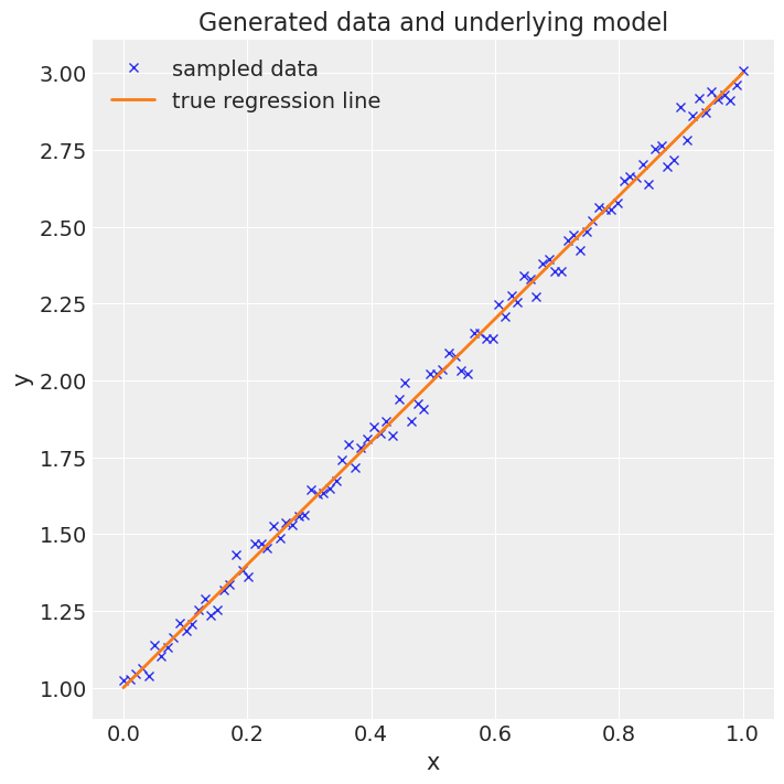
设置参数并使用线性模型生成数据#
# set up the model and data
np.random.seed(RANDOM_SEED)
size = 100
true_intercept = 1
true_slope = 2
sigma = 0.2
x = np.linspace(0, 1, size)

# y = a + b*x
true_regression_line = true_intercept + true_slope * x

# add noise
y = true_regression_line + np.random.normal(0, sigma**2, size)
s = sigma

# reduced datasets
# We use fewer data in the coarse models compared to the fine model in order to make them less accurate
x_coarse_0 = x[::3]
y_coarse_0 = y[::3]
x_coarse_1 = x[::2]
y_coarse_1 = y[::2]

# MCMC parameters
ndraws = 3000
ntune = 1000
nsub = 5
nchains = 2
# Plot the data
fig = plt.figure(figsize=(7, 7))
ax = fig.add_subplot(111, xlabel="x", ylabel="y", title="Generated data and underlying model")
ax.plot(x, y, "x", label="sampled data")
ax.plot(x, true_regression_line, label="true regression line", lw=2.0)
plt.legend(loc=0);
创建一个实现似然的theano操作#
为了使用方差减少,用户需要定义一个Theano Op来计算正向模型(或正向模型和似然函数)。
此外,此Op需要将感兴趣的量保存到一个名为Q的模型变量中。
这里我们使用一个包含正向模型(即在这种情况下为线性方程)和似然计算的Theano Op。感兴趣的量通过perform()函数计算,它是给定theta的所有数据点的线性预测的平均值。
class Likelihood(tt.Op):
    # Specify what type of object will be passed and returned to the Op when it is
    # called. In our case we will be passing it a vector of values (the parameters
    # that define our model) and returning a scalar (likelihood)
    itypes = [tt.dvector]
    otypes = [tt.dscalar]

    def __init__(self, x, y, pymc3_model):
        """
        Initialise the Op with various things that our likelihood requires.
        Parameters
        ----------
        x:
            The x points.
        y:
            The y points.
        pymc3_model:
            The pymc3 model.
        """
        self.x = x
        self.y = y
        self.pymc3_model = pymc3_model

    def perform(self, node, inputs, outputs):
        intercept = inputs[0][0]
        x_coeff = inputs[0][1]

        # this uses the linear model to calculate outputs
        temp = intercept + x_coeff * self.x
        # this saves the quantity of interest to the pymc3 model variable Q
        self.pymc3_model.Q.set_value(temp.mean())
        # this calculates the likelihood value
        outputs[0][0] = np.array(-(0.5 / s**2) * np.sum((temp - self.y) ** 2))
定义粗略模型#
在这里,我们为MLDA创建粗略模型。
我们需要在每个模型中包含一个pm.Data()变量Q,初始化为0.0。这些变量在perform()下的Op代码运行时在采样期间设置。
mout = []
coarse_models = []

# Set up models in pymc3 for each level - excluding finest model level
# Level 0 (coarsest)
with pm.Model() as coarse_model_0:
    # A variable Q has to be defined if you want to use the variance reduction feature
    # Q can be of any dimension - here it a scalar
    Q = pm.Data("Q", np.float(0.0))

    # Define priors
    intercept = pm.Normal("Intercept", 0, sigma=20)
    x_coeff = pm.Normal("x", 0, sigma=20)

    # convert thetas to a tensor vector
    theta = tt.as_tensor_variable([intercept, x_coeff])

    # Here we instantiate a Likelihood object using the class defined above
    # and we add to the mout list. We pass the coarse data x_coarse_0 and y_coarse_0
    # and the coarse pymc3 model coarse_model_0. This creates a coarse likelihood.
    mout.append(Likelihood(x_coarse_0, y_coarse_0, coarse_model_0))

    # This uses the likelihood object to define the likelihood of the model, given theta
    pm.Potential("likelihood", mout[0](theta))

    coarse_models.append(coarse_model_0)

# Level 1
with pm.Model() as coarse_model_1:
    # A variable Q has to be defined if you want to use the variance reduction feature
    # Q can be of any dimension - here it a scalar
    Q = pm.Data("Q", np.float64(0.0))

    # Define priors
    intercept = pm.Normal("Intercept", 0, sigma=20)
    x_coeff = pm.Normal("x", 0, sigma=20)

    # convert thetas to a tensor vector
    theta = tt.as_tensor_variable([intercept, x_coeff])

    # Here we instantiate a Likelihood object using the class defined above
    # and we add to the mout list. We pass the coarse data x_coarse_1 and y_coarse_1
    # and the coarse pymc3 model coarse_model_1. This creates a coarse likelihood.
    mout.append(Likelihood(x_coarse_1, y_coarse_1, coarse_model_1))

    # This uses the likelihood object to define the likelihood of the model, given theta
    pm.Potential("likelihood", mout[1](theta))

    coarse_models.append(coarse_model_1)
<ipython-input-6-18d173b4fdbe>:9: DeprecationWarning: `np.float` is a deprecated alias for the builtin `float`. To silence this warning, use `float` by itself. Doing this will not modify any behavior and is safe. If you specifically wanted the numpy scalar type, use `np.float64` here.
Deprecated in NumPy 1.20; for more details and guidance: https://numpy.org/devdocs/release/1.20.0-notes.html#deprecations
  Q = pm.Data("Q", np.float(0.0))
<ipython-input-6-18d173b4fdbe>:32: DeprecationWarning: `np.float` is a deprecated alias for the builtin `float`. To silence this warning, use `float` by itself. Doing this will not modify any behavior and is safe. If you specifically wanted the numpy scalar type, use `np.float64` here.
Deprecated in NumPy 1.20; for more details and guidance: https://numpy.org/devdocs/release/1.20.0-notes.html#deprecations
  Q = pm.Data("Q", np.float(0.0))
定义精细模型和样本#
这里我们定义了精细(即正确)的模型,并使用MLDA(有无方差减少)从中进行采样。
注意,这里也使用了Q。
我们创建了两个MLDA采样器,一个启用了VR,另一个没有启用。
with pm.Model() as model:
    # A variable Q has to be defined if you want to use the variance reduction feature
    # Q can be of any dimension - here it a scalar
    Q = pm.Data("Q", np.float64(0.0))

    # Define priors
    intercept = pm.Normal("Intercept", 0, sigma=20)
    x_coeff = pm.Normal("x", 0, sigma=20)

    # convert thetas to a tensor vector
    theta = tt.as_tensor_variable([intercept, x_coeff])

    # Here we instantiate a Likelihood object using the class defined above
    # and we add to the mout list. We pass the fine data x and y
    # and the fine pymc3 model model. This creates a fine likelihood.
    mout.append(Likelihood(x, y, model))

    # This uses the likelihood object to define the likelihood of the model, given theta
    pm.Potential("likelihood", mout[-1](theta))

    # MLDA with variance reduction
    step_with = pm.MLDA(
        coarse_models=coarse_models, subsampling_rates=nsub, variance_reduction=True
    )

    # MLDA without variance reduction
    step_without = pm.MLDA(
        coarse_models=coarse_models,
        subsampling_rates=nsub,
        variance_reduction=False,
        store_Q_fine=True,
    )

    # sample
    trace1 = pm.sample(
        draws=ndraws,
        step=step_with,
        chains=nchains,
        tune=ntune,
        discard_tuned_samples=True,
        random_seed=RANDOM_SEED,
        cores=1,
    )

    trace2 = pm.sample(
        draws=ndraws,
        step=step_without,
        chains=nchains,
        tune=ntune,
        discard_tuned_samples=True,
        random_seed=RANDOM_SEED,
        cores=1,
    )
Sequential sampling (2 chains in 1 job)
MLDA: [x, Intercept]
/Users/CloudChaoszero/Documents/Projects-Dev/pymc3/pymc3/step_methods/mlda.py:771: RuntimeWarning: overflow encountered in exp
  stats = {"tune": self.tune, "accept": np.exp(accept), "accepted": accepted}
/Users/CloudChaoszero/Documents/Projects-Dev/pymc3/pymc3/sampling.py:465: FutureWarning: In an upcoming release, pm.sample will return an `arviz.InferenceData` object instead of a `MultiTrace` by default. You can pass return_inferencedata=True or return_inferencedata=False to be safe and silence this warning.
  warnings.warn(
/Users/CloudChaoszero/Documents/Projects-Dev/pymc3/pymc3/step_methods/mlda.py:771: RuntimeWarning: overflow encountered in exp
  stats = {"tune": self.tune, "accept": np.exp(accept), "accepted": accepted}
显示统计摘要#
with model:
    trace1_az = az.from_pymc3(trace1)
az.summary(trace1_az)
| mean | sd | hdi_3% | hdi_97% | mcse_mean | mcse_sd | ess_mean | ess_sd | ess_bulk | ess_tail | r_hat | |
|---|---|---|---|---|---|---|---|---|---|---|---|
| Intercept | 1.002 | 0.039 | 0.933 | 1.080 | 0.001 | 0.001 | 2487.0 | 2481.0 | 2501.0 | 2887.0 | 1.0 |
| x | 1.996 | 0.067 | 1.875 | 2.123 | 0.001 | 0.001 | 2535.0 | 2535.0 | 2536.0 | 2862.0 | 1.0 |
with model:
    trace2_az = az.from_pymc3(trace2)
az.summary(trace2_az)
| mean | sd | hdi_3% | hdi_97% | mcse_mean | mcse_sd | ess_mean | ess_sd | ess_bulk | ess_tail | r_hat | |
|---|---|---|---|---|---|---|---|---|---|---|---|
| Intercept | 1.002 | 0.041 | 0.924 | 1.075 | 0.001 | 0.001 | 3206.0 | 3206.0 | 3186.0 | 3919.0 | 1.0 |
| x | 1.997 | 0.070 | 1.866 | 2.127 | 0.001 | 0.001 | 3264.0 | 3255.0 | 3263.0 | 3773.0 | 1.0 |
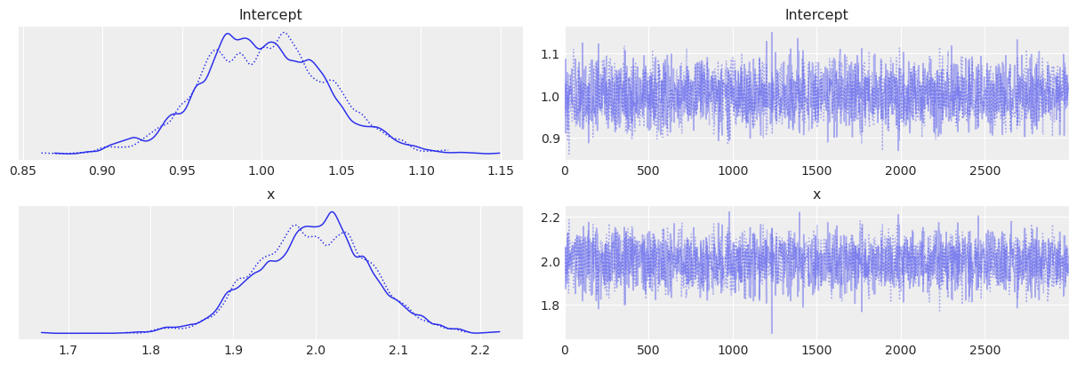
显示轨迹图#
az.plot_trace(trace1_az)
array([[<AxesSubplot:title={'center':'Intercept'}>,
        <AxesSubplot:title={'center':'Intercept'}>],
       [<AxesSubplot:title={'center':'x'}>,
        <AxesSubplot:title={'center':'x'}>]], dtype=object)
az.plot_trace(trace1_az)
array([[<AxesSubplot:title={'center':'Intercept'}>,
        <AxesSubplot:title={'center':'Intercept'}>],
       [<AxesSubplot:title={'center':'x'}>,
        <AxesSubplot:title={'center':'x'}>]], dtype=object)
估计两种方法的标准误差#
比较Q估计的标准误差:
标准方法:仅使用细链中的Q值(Q_2)- 不带VR的MLDA采样
折叠求和(VR)方法:使用最粗链的Q值(Q_0),加上所有层级之间的差异估计(在这种情况下是Q_1_0和Q_2_1) - 来自MLDA与VR的样本
0) 用于感兴趣数量估计的便利函数#
从轨迹中直接提取折叠求和(VR)方法的感兴趣量的期望值和标准误差的最简单方法是使用extract_Q_estimate(...)函数,如下所示。
在本笔记本的剩余部分中,我们详细演示了不使用此便捷函数的提取过程。
Q_expectation, Q_SE = pm.step_methods.mlda.extract_Q_estimate(trace=trace1, levels=3)
print(Q_expectation, Q_SE)
2.0005638367325767 0.00022441567873480883
1) 从轨迹中提取感兴趣的数量#
这需要使用numpy进行一些重塑。请注意,我们将所有链的样本追加到一个长数组中。
# MLDA without VR
Q_2 = trace2.get_sampler_stats("Q_2").reshape((1, nchains * ndraws))

# MLDA with VR
Q_0 = np.concatenate(trace1.get_sampler_stats("Q_0")).reshape((1, nchains * ndraws * nsub * nsub))
Q_1_0 = np.concatenate(trace1.get_sampler_stats("Q_1_0")).reshape((1, nchains * ndraws * nsub))
Q_2_1 = np.concatenate(trace1.get_sampler_stats("Q_2_1")).reshape((1, nchains * ndraws))

# Estimates
Q_mean_standard = Q_2.mean()
Q_mean_vr = Q_0.mean() + Q_1_0.mean() + Q_2_1.mean()

print(f"Q_0 mean = {Q_0.mean()}")
print(f"Q_1_0 mean = {Q_1_0.mean()}")
print(f"Q_2_1 mean = {Q_2_1.mean()}")
print(f"Q_2 mean = {Q_2.mean()}")
print(f"Standard method:    Mean: {Q_mean_standard}")
print(f"VR method:    Mean: {Q_mean_vr}")
Q_0 mean = 2.000553055055296
Q_1_0 mean = -0.010069727227140116
Q_2_1 mean = 0.010080508904420811
Q_2 mean = 1.9999261715750685
Standard method:    Mean: 1.9999261715750685
VR method:    Mean: 2.0005638367325767
计算Q数量样本的方差#
这表明差异的方差比任何链的方差都要小几个数量级
Q_2.var()
0.000414235279421214
Q_0.var()
0.0010760873150945423
Q_1_0.var()
2.3175382954631006e-07
Q_2_1.var()
1.1469959605972495e-07
使用ESS计算每个项的标准误差#
ess_Q0 = az.ess(np.array(Q_0, np.float64))
ess_Q_1_0 = az.ess(np.array(Q_1_0, np.float64))
ess_Q_2_1 = az.ess(np.array(Q_2_1, np.float64))
ess_Q2 = az.ess(np.array(Q_2, np.float64))
# note that the chain in level 2 has much fewer samples than the chain in level 0 (because of the subsampling rates)
print(ess_Q2, ess_Q0, ess_Q_1_0, ess_Q_2_1)
3583.1266973140664 21397.989450048717 8294.638940009752 2533.2315562978047
标准误差通过 \(Var(Q) \over ESS(Q)\) 估计。 很明显,差异的标准误差远低于水平 0 和 2
Q_2.var() / ess_Q2
1.156072096841363e-07
Q_0.var() / ess_Q0
5.0289178691603306e-08
Q_1_0.var() / ess_Q_1_0
2.7940195013001685e-11
Q_2_1.var() / ess_Q_2_1
4.5277975388618976e-11
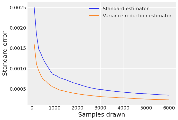
计算两个竞争估计量在不同样本块中的总标准误差#
该图展示了当我们收集更多样本时误差的衰减情况,证明了VR技术在减少标准误差方面的优势。
step = 100

Q2_SE = np.zeros(int(nchains * ndraws / step))
Q0_SE = np.zeros(int(nchains * ndraws / step))
Q_1_0_SE = np.zeros(int(nchains * ndraws / step))
Q_2_1_SE = np.zeros(int(nchains * ndraws / step))
E_standard_SE = np.zeros(int(nchains * ndraws / step))
E_VR_SE = np.zeros(int(nchains * ndraws / step))
k = 0

for i in np.arange(step, nchains * ndraws + 1, step):
    Q2_SE[k] = Q_2[0, 0:i].var() / az.ess(np.array(Q_2[0, 0:i], np.float64))
    Q0_SE[k] = Q_0[0, 0 : i * (nsub**2)].var() / az.ess(
        np.array(Q_0[0, 0 : i * (nsub**2)], np.float64)
    )
    Q_1_0_SE[k] = Q_1_0[0, 0 : i * nsub].var() / az.ess(
        np.array(Q_1_0[0, 0 : i * nsub], np.float64)
    )
    Q_2_1_SE[k] = Q_2_1[0, 0:i].var() / az.ess(np.array(Q_2_1[0, 0:i], np.float64))
    E_standard_SE[k] = np.sqrt(Q2_SE[k])
    E_VR_SE[k] = np.sqrt(Q0_SE[k] + Q_1_0_SE[k] + Q_2_1_SE[k])
    k += 1

fig = plt.figure()
ax = fig.gca()

for axis in [ax.yaxis]:
    axis.set_major_formatter(ScalarFormatter())

ax.plot(np.arange(step, nchains * ndraws + 1, step), E_standard_SE)
ax.plot(np.arange(step, nchains * ndraws + 1, step), E_VR_SE)
plt.xlabel("Samples drawn", fontsize=18)
plt.ylabel("Standard error", fontsize=18)
ax.legend(["Standard estimator", "Variance reduction estimator"])
plt.show()
%load_ext watermark
%watermark -n -u -v -iv -w
Last updated: Sat Feb 06 2021

Python implementation: CPython
Python version       : 3.8.6
IPython version      : 7.20.0

theano    : 1.1.2
arviz     : 0.11.0
sys       : 3.8.6 | packaged by conda-forge | (default, Jan 25 2021, 23:22:12)
[Clang 11.0.1 ]
matplotlib: None
numpy     : 1.20.0
pymc3     : 3.11.0

Watermark: 2.1.0