


冈比亚疟疾的流行#
导入#
import arviz as az
import matplotlib.pyplot as plt
import numpy as np
import pandas as pd
import pymc as pm
import pytensor.tensor as pt
注意
本笔记本使用了不是 PyMC 依赖项的库,因此需要专门安装这些库才能运行此笔记本。打开下面的下拉菜单以获取更多指导。
Extra dependencies install instructions
为了在本地或binder上运行此笔记本,您不仅需要一个安装了所有可选依赖项的PyMC工作环境,还需要安装一些额外的依赖项。有关安装PyMC本身的建议,请参阅安装
您可以使用您喜欢的包管理器安装这些依赖项,我们提供了以下作为示例的pip和conda命令。
$ pip install
请注意,如果您想(或需要)从笔记本内部而不是命令行安装软件包,您可以通过运行pip命令的变体来安装软件包:
导入系统
!{sys.executable} -m pip install
您不应运行!pip install,因为它可能会在不同的环境中安装包,即使安装了也无法从Jupyter笔记本中使用。
另一个替代方案是使用conda:
$ conda 安装
在安装科学计算Python包时,我们推荐使用conda forge
# These dependencies need to be installed separately from PyMC
import folium
import geopandas as gpd
import mapclassify
import rasterio as rio

from pyproj import Transformer
介绍#
通常,我们发现自己拥有一组空间相关的连续测量数据(地统计数据),我们的目标是确定在未采样的周围区域中该测量的估计值。在下面的案例研究中,我们研究了冈比亚地区65个村庄中检测出疟疾阳性的个体数量,并继续估计这65个采样村庄周围区域内的疟疾流行率(总阳性数/总检测人数)。
数据处理#
# load the tabular data
try:
    gambia = pd.read_csv("../data/gambia_dataset.csv")
except FileNotFoundError:
    gambia = pd.read_csv(pm.get_data("gambia_dataset.csv"))
gambia.head()
| Unnamed: 0 | x | y | pos | age | netuse | treated | green | phc | |
|---|---|---|---|---|---|---|---|---|---|
| 0 | 1850 | 349631.3 | 1458055 | 1 | 1783 | 0 | 0 | 40.85 | 1 |
| 1 | 1851 | 349631.3 | 1458055 | 0 | 404 | 1 | 0 | 40.85 | 1 |
| 2 | 1852 | 349631.3 | 1458055 | 0 | 452 | 1 | 0 | 40.85 | 1 |
| 3 | 1853 | 349631.3 | 1458055 | 1 | 566 | 1 | 0 | 40.85 | 1 |
| 4 | 1854 | 349631.3 | 1458055 | 0 | 598 | 1 | 0 | 40.85 | 1 |
数据目前是按个人级别存储的,但为了我们的目的,我们需要将其转换为村庄级别。我们将按村庄汇总数据,以计算检测的总人数、检测呈阳性的人数以及样本的阳性率;该阳性率将通过将检测呈阳性的总人数除以检测的总人数来计算。
# For each village compute the total tested, total positive, and the prevalence
gambia_agg = (
    gambia.groupby(["x", "y"])
    .agg(total=("x", "size"), positive=("pos", "sum"))
    .eval("prev = positive / total")
    .reset_index()
)
gambia_agg.head()
| x | y | total | positive | prev | |
|---|---|---|---|---|---|
| 0 | 349631.3 | 1458055 | 33 | 17 | 0.515152 |
| 1 | 358543.1 | 1460112 | 63 | 19 | 0.301587 |
| 2 | 360308.1 | 1460026 | 17 | 7 | 0.411765 |
| 3 | 363795.7 | 1496919 | 24 | 8 | 0.333333 |
| 4 | 366400.5 | 1460248 | 26 | 10 | 0.384615 |
我们需要将我们的数据框转换为地理数据框。为此,我们需要知道要使用哪种坐标参考系统(CRS),无论是地理坐标系统(GCS)还是投影坐标系统(PCS)。GCS告诉你数据在地球上的位置,而PCS告诉你如何在二维平面上绘制数据。有许多不同的GCS/PCS,因为每个GCS/PCS都是地球表面的模型。然而,地球表面在不同位置之间是变化的。因此,不同的GCS/PCS版本将根据你的分析所基于的地理位置而更加准确。由于我们的分析是在冈比亚进行的,我们将使用PCS EPSG 32628 和GCS EPSG 4326 在地球上绘图。其中EPSG代表欧洲石油调查组,这是一个维护坐标系统大地测量参数的组织。
# Create a GeoDataframe and set coordinate reference system to EPSG 4326
gambia_gpdf = gpd.GeoDataFrame(
    gambia_agg, geometry=gpd.points_from_xy(gambia_agg["x"], gambia_agg["y"]), crs="EPSG:32628"
).drop(["x", "y"], axis=1)

gambia_gpdf_4326 = gambia_gpdf.to_crs(crs="EPSG:4326")
# Get an interactive plot of the data with a cmap on the prevalence values
gambia_gpdf_4326.round(2).explore(column="prev")
我们希望在我们的地图上包含冈比亚的 elevations。为此,我们从栅格文件中提取 elevation 值并将其叠加在地图上。颜色较深的红色区域表示较高的 elevation。
# Overlay the raster image of elevations in the Gambia on top of the map
m = gambia_gpdf_4326.round(2).explore(column="prev")

## Load the elevation rasterfile
in_path = "../data/GMB_elv_msk.tif"

dst_crs = "EPSG:4326"

with rio.open(in_path) as src:

    img = src.read()

    src_crs = src.crs["init"].upper()
    min_lon, min_lat, max_lon, max_lat = src.bounds
    xs = gambia_gpdf_4326["geometry"].x
    ys = gambia_gpdf_4326["geometry"].y
    rows, cols = rio.transform.rowcol(src.transform, xs, ys)

## Conversion of elevation locations from UTM to WGS84 CRS
bounds_orig = [[min_lat, min_lon], [max_lat, max_lon]]

bounds_fin = []

for item in bounds_orig:
    # converting to lat/lon
    lat = item[0]
    lon = item[1]

    proj = Transformer.from_crs(
        int(src_crs.split(":")[1]), int(dst_crs.split(":")[1]), always_xy=True
    )

    lon_n, lat_n = proj.transform(lon, lat)

    bounds_fin.append([lat_n, lon_n])

# Finding the center of latitude & longitude
centre_lon = bounds_fin[0][1] + (bounds_fin[1][1] - bounds_fin[0][1]) / 2
centre_lat = bounds_fin[0][0] + (bounds_fin[1][0] - bounds_fin[0][0]) / 2

# Overlay raster
m.add_child(
    folium.raster_layers.ImageOverlay(
        img.transpose(1, 2, 0),
        opacity=0.7,
        bounds=bounds_fin,
        overlay=True,
        control=True,
        cross_origin=False,
        zindex=1,
        colormap=lambda x: (1, 0, 0, x),
    )
)

m
/opt/miniconda3/envs/pymc_examples_contrib/lib/python3.12/site-packages/branca/utilities.py:320: RuntimeWarning: invalid value encountered in cast
  array = array.astype("uint8")
我们希望在模型中将海拔作为协变量。因此,我们需要从栅格图像中提取值并将其存储到数据框中。
# Pull the elevation values from the raster file and put them into a dataframe
path = "../data/GMB_elv_msk.tif"

with rio.open(path) as f:
    arr = f.read(1)
    mask = arr != f.nodata
    elev = arr[mask]
    col, row = np.where(mask)
    x, y = f.xy(col, row)
    uid = np.arange(f.height * f.width).reshape((f.height, f.width))[mask]

result = np.rec.fromarrays([uid, x, y, elev], names=["id", "x", "y", "elev"])
elevations = pd.DataFrame(result)
elevations = gpd.GeoDataFrame(
    elevations, geometry=gpd.points_from_xy(elevations["x"], elevations["y"], crs="EPSG:4326")
)
提取高程值后,我们需要对包含患病率的聚合数据集执行空间连接。空间连接是一种基于地理信息进行连接的特殊连接。在执行此类连接时,使用适合您地理区域的投影坐标系统至关重要。
# Set coordinate system to EPSG 32628 and spatially join our prevalence dataframe to our elevations dataframe
elevations = elevations.to_crs(epsg="32628")
gambia_gpdf = gambia_gpdf.sjoin_nearest(elevations, how="inner")
# Set CRS to EPSG 4326 for plotting
gambia_gpdf_4326 = gambia_gpdf.to_crs(crs="EPSG:4326")
gambia_gpdf_4326.head()
| total | positive | prev | geometry | index_right | id | x | y | elev | |
|---|---|---|---|---|---|---|---|---|---|
| 0 | 33 | 17 | 0.515152 | POINT (-16.38755 13.18541) | 12390 | 39649 | -16.387500 | 13.187500 | 15.0 |
| 1 | 63 | 19 | 0.301587 | POINT (-16.30543 13.20444) | 12166 | 38843 | -16.304167 | 13.204167 | 33.0 |
| 2 | 17 | 7 | 0.411765 | POINT (-16.28914 13.20374) | 12168 | 38845 | -16.287500 | 13.204167 | 32.0 |
| 3 | 24 | 8 | 0.333333 | POINT (-16.25869 13.53742) | 3429 | 22528 | -16.262500 | 13.537500 | 20.0 |
| 4 | 26 | 10 | 0.384615 | POINT (-16.23294 13.20603) | 12175 | 38852 | -16.229167 | 13.204167 | 29.0 |
# Get relevant measures for modeling
elev = gambia_gpdf["elev"].values
pos = gambia_gpdf["positive"].values
n = gambia_gpdf["total"].values
lonlat = gambia_gpdf[["y", "x"]].values
# Set a seed for reproducibility of results
seed: int = sum(map(ord, "spatialmalaria"))
rng: np.random.Generator = np.random.default_rng(seed=seed)
模型规范#
我们指定以下模型:
其中 \(n_{i}\) 表示一个接受疟疾检测的个体,\(P(x_{i})\) 是位置 \(x_{i}\) 处的疟疾流行率,\(\beta_{0}\) 是截距,\(\beta_{1}\) 是高程协变量的系数,\(S(x_{i})\) 是一个具有 Matérn 协方差函数的零均值高斯过程,其 \(\nu=\frac{3}{2}\),我们将使用 Hilbert 空间高斯过程 (HSGP) 对其进行近似。
为了使用HSGP近似高斯过程,我们需要选择参数m和c。要了解更多关于如何设置这些参数的信息,请参考这个精彩的示例,了解如何设置这些参数。
with pm.Model() as hsgp_model:
    _X = pm.Data("X", lonlat)
    _elev = pm.Data("elevation", elev_std)

    ls = pm.Gamma("ls", mu=20, sigma=5)
    cov_func = pm.gp.cov.Matern32(2, ls=ls)
    m0, m1, c = 40, 40, 2.5
    gp = pm.gp.HSGP(m=[m0, m1], c=c, cov_func=cov_func)
    s = gp.prior("s", X=_X)

    beta_0 = pm.Normal("beta_0", 0, 1)
    beta_1 = pm.Normal("beta_1", 0, 1)

    p_logit = pm.Deterministic("p_logit", beta_0 + beta_1 * _elev + s)
    p = pm.Deterministic("p", pm.math.invlogit(p_logit))
    pm.Binomial("likelihood", n=n, logit_p=p_logit, observed=pos)
hsgp_model.to_graphviz()

2024-08-28 15:12:41.392183: E external/xla/xla/service/slow_operation_alarm.cc:65] Constant folding an instruction is taking > 1s:

  %reduce = f64[4,1000,1600,1]{3,2,1,0} reduce(f64[4,1000,1,1600,1]{4,3,2,1,0} %broadcast.9, f64[] %constant.15), dimensions={2}, to_apply=%region_1.42, metadata={op_name="jit(process_fn)/jit(main)/reduce_prod[axes=(2,)]" source_file="/var/folders/h_/9hc6pmt169bdm70pz7z4s9rm0000gn/T/tmpuppt4vln" source_line=25}

This isn't necessarily a bug; constant-folding is inherently a trade-off between compilation time and speed at runtime. XLA has some guards that attempt to keep constant folding from taking too long, but fundamentally you'll always be able to come up with an input program that takes a long time.

If you'd like to file a bug, run with envvar XLA_FLAGS=--xla_dump_to=/tmp/foo and attach the results.
2024-08-28 15:13:04.025470: E external/xla/xla/service/slow_operation_alarm.cc:133] The operation took 23.638298s
Constant folding an instruction is taking > 1s:

  %reduce = f64[4,1000,1600,1]{3,2,1,0} reduce(f64[4,1000,1,1600,1]{4,3,2,1,0} %broadcast.9, f64[] %constant.15), dimensions={2}, to_apply=%region_1.42, metadata={op_name="jit(process_fn)/jit(main)/reduce_prod[axes=(2,)]" source_file="/var/folders/h_/9hc6pmt169bdm70pz7z4s9rm0000gn/T/tmpuppt4vln" source_line=25}

This isn't necessarily a bug; constant-folding is inherently a trade-off between compilation time and speed at runtime. XLA has some guards that attempt to keep constant folding from taking too long, but fundamentally you'll always be able to come up with an input program that takes a long time.

If you'd like to file a bug, run with envvar XLA_FLAGS=--xla_dump_to=/tmp/foo and attach the results.
长度尺度的后验均值为0.21(如下所示)。因此,我们可以预期高斯均值会随着我们远离地图上任何采样点0.21度而衰减至0(因为我们设置了0均值函数)。尽管由于长度尺度不受观测数据约束,这不是一个严格的截止点,但能够直观地理解长度尺度如何影响估计仍然是有用的。
az.summary(hsgp_trace, var_names=["ls"], kind="stats")
| mean | sd | hdi_3% | hdi_97% | |
|---|---|---|---|---|
| ls | 0.205 | 0.166 | 0.113 | 0.285 |
后验预测检查#
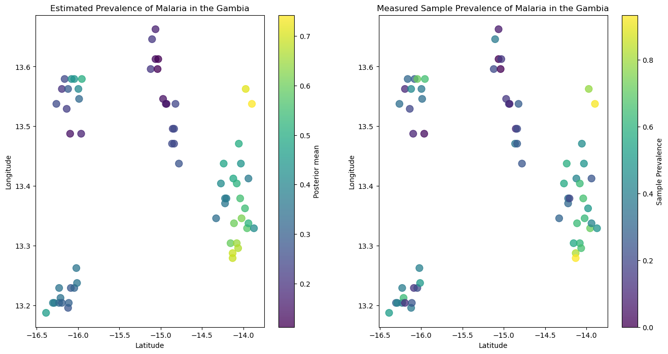
我们需要验证我们的模型规范是否正确地表示了观测数据。我们可以推出患病率的后验预测,并在坐标系上绘制它们,以检查它们是否与样本中的观测患病率相似
with hsgp_model:
    ppc = pm.sample_posterior_predictive(hsgp_trace, random_seed=rng)
Sampling: [likelihood]
posterior_prevalence = hsgp_trace["posterior"]["p"]
我们可以看到,在下图中左侧的后验预测与右侧显示的观测样本一致。
plt.subplots(nrows=1, ncols=2, figsize=(16, 8))
plt.subplot(1, 2, 1)

plt.scatter(
    lonlat[:, 1],
    lonlat[:, 0],
    c=posterior_prevalence.mean(("chain", "draw")),
    marker="o",
    alpha=0.75,
    s=100,
    edgecolor=None,
)
plt.xlabel("Latitude")
plt.ylabel("Longitude")
plt.title("Estimated Prevalence of Malaria in the Gambia")
plt.colorbar(label="Posterior mean")

plt.subplot(1, 2, 2)

plt.scatter(
    lonlat[:, 1],
    lonlat[:, 0],
    c=gambia_gpdf_4326["prev"],
    marker="o",
    alpha=0.75,
    s=100,
    edgecolor=None,
)
plt.xlabel("Latitude")
plt.ylabel("Longitude")
plt.title("Measured Sample Prevalence of Malaria in the Gambia")
plt.colorbar(label="Sample Prevalence");
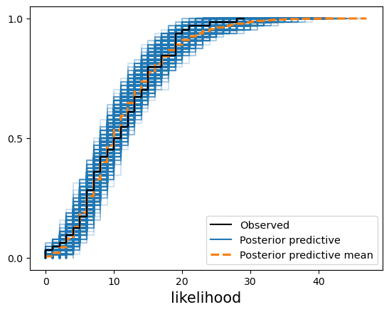
我们还可以检查似然性(检测出疟疾阳性的个体数量)是否与观测数据一致。正如您在下图中看到的,我们的后验预测样本能够代表观测样本。
az.plot_ppc(ppc, kind="cumulative");
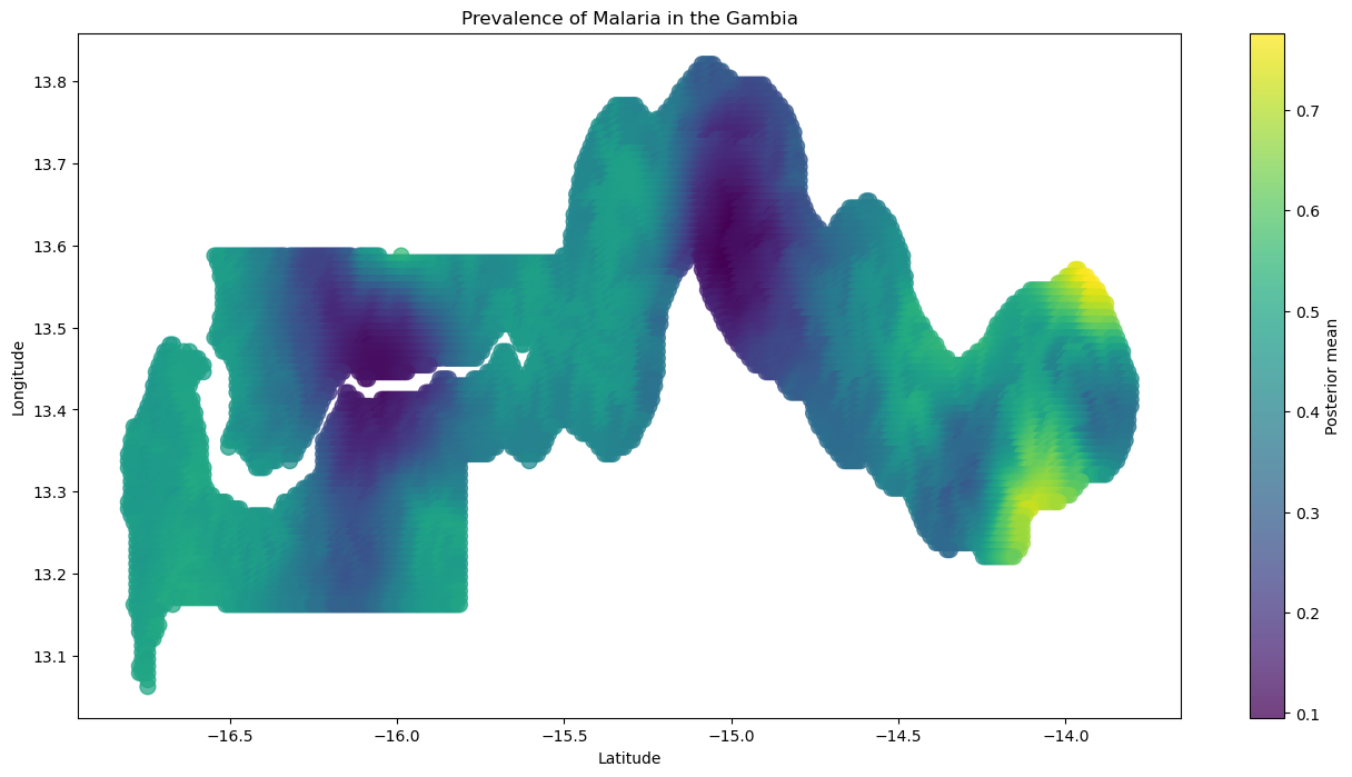
样本外后验预测#
现在我们已经验证了我们有一个收敛的代表性模型,我们希望估计在我们观察到数据点的周围地区疟疾的流行情况。我们的新数据集将包括冈比亚内每个经纬度位置,我们在那里有一个高程的测量值。
with hsgp_model:
    pm.set_data(new_data={"X": new_lonlat, "elevation": new_elev_std})
    pp = pm.sample_posterior_predictive(hsgp_trace, var_names=["p"], random_seed=rng)
Sampling: []
posterior_predictive_prevalence = pp["posterior_predictive"]["p"]
我们可以绘制样本外后验预测图,以可视化冈比亚疟疾患病率的估计值。在下图中,您会注意到,在我们观察到数据的区域周围,患病率有一个平滑的过渡,较近的区域患病率更相似,随着距离的增加,患病率趋近于零(高斯过程的均值)。
fig = plt.figure(figsize=(16, 8))

plt.scatter(
    new_lonlat[:, 1],
    new_lonlat[:, 0],
    c=posterior_predictive_prevalence.mean(("chain", "draw")),
    marker="o",
    alpha=0.75,
    s=100,
    edgecolor=None,
)
plt.xlabel("Latitude")
plt.ylabel("Longitude")
plt.title("Prevalence of Malaria in the Gambia")
plt.colorbar(label="Posterior mean");
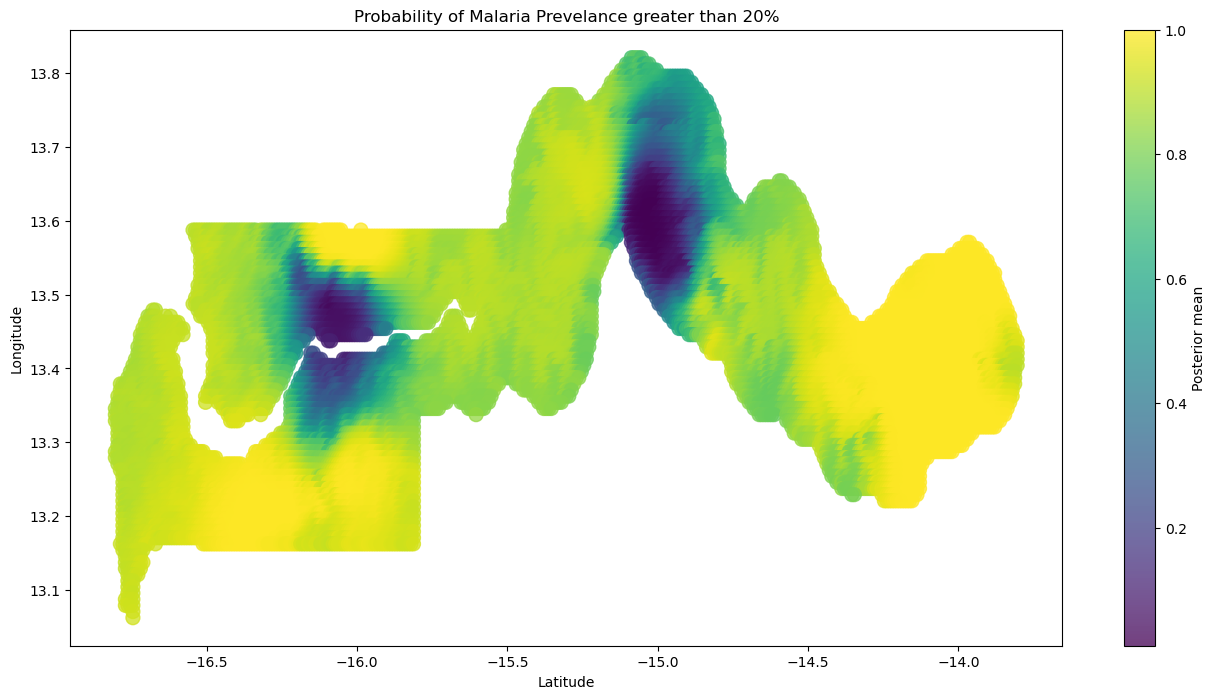
基于超限概率的决策#
确定我们可能决定实施干预措施的一个方法是查看某些选定疟疾流行率阈值的超额概率。这些超额概率将使我们能够将我们对估计流行率的不确定性纳入考虑,而不仅仅是考虑后验分布的均值。在我们的用例中,我们决定将流行率的超额阈值设定为20%。
prob_prev_gt_20percent = 1 - (posterior_predictive_prevalence <= 0.2).mean(("chain", "draw"))
我们可以利用从下图获得的见解,向我们最有信心疟疾流行率超过20%的地区发送援助。
fig = plt.figure(figsize=(16, 8))

plt.scatter(
    new_lonlat[:, 1],
    new_lonlat[:, 0],
    c=prob_prev_gt_20percent,
    marker="o",
    alpha=0.75,
    s=100,
    edgecolor=None,
)
plt.xlabel("Latitude")
plt.ylabel("Longitude")
plt.title("Probability of Malaria Prevelance greater than 20%")
plt.colorbar(label="Posterior mean");
不同的协方差函数#
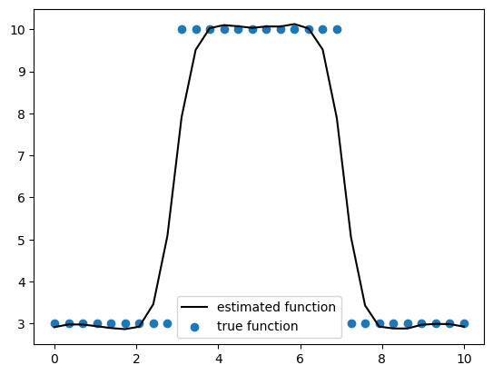
在我们结束之前,让我们简要讨论一下为什么我们决定使用Matérn协方差函数族而不是指数二次方。Matérn协方差族是指数二次方协方差的一般化。当Matérn的平滑参数\(\nu \to \infty\)时,我们得到指数二次方协方差函数。随着平滑参数的增加,您正在估计的函数变得更加平滑。一些常用的\(\nu\)值是\(\frac{1}{2}\)、\(\frac{3}{2}\)和\(\frac{5}{2}\)。通常,在估计具有空间依赖性的测量时,我们不希望过于平滑的函数,因为这会阻止我们的估计捕捉到我们正在估计的测量中的突然变化。下面我们模拟一些数据来展示Matérn如何能够捕捉这些突然变化,而指数二次方则过于平滑。为了简单起见,我们将在一维中工作,但这些概念适用于二维数据。
# simulate 1-dimensional data
x = np.linspace(0, 10, 30)
y = list()
for v in x:
    # introduce abrupt changes
    if v > 3 and v < 7:
        y.append(np.array(10.0))
    else:
        y.append(np.array(3.0))
y = np.array(y).ravel()
# Fit a GP to model the simulated data
with pm.Model() as matern_model:

    eta = pm.Exponential("eta", scale=10.0)
    ls = pm.Lognormal("ls", mu=0.5, sigma=0.75)
    cov_func = eta**2 * pm.gp.cov.Matern32(input_dim=1, ls=ls)
    gp = pm.gp.Latent(cov_func=cov_func)
    s = gp.prior("s", X=x[:, None])

    measurement_error = pm.Exponential("measurement_error", scale=5.0)
    pm.Normal("likelihood", mu=s, sigma=measurement_error, observed=y)
    matern_idata = pm.sample(
        draws=2000, tune=2000, nuts_sampler="numpyro", target_accept=0.98, random_seed=rng
    )
There were 2 divergences after tuning. Increase `target_accept` or reparameterize.
with matern_model:
    ppc = pm.sample_posterior_predictive(matern_idata, random_seed=rng)
Sampling: [likelihood]
y_mean_ppc = ppc["posterior_predictive"]["likelihood"].mean(("chain", "draw"))
# Plot the estimated function against the true function
plt.plot(x, y_mean_ppc, c="k", label="estimated function")
plt.scatter(x, y, label="true function")
plt.legend(loc="best")
<matplotlib.legend.Legend at 0x31f703ce0>
# Fit a GP to model the simulated data
with pm.Model() as expquad_model:

    eta = pm.Exponential("eta", scale=10.0)
    ls = pm.Lognormal("ls", mu=0.5, sigma=0.75)
    cov_func = eta**2 * pm.gp.cov.ExpQuad(input_dim=1, ls=ls)
    gp = pm.gp.Latent(cov_func=cov_func)
    s = gp.prior("s", X=x[:, None])

    measurement_error = pm.Exponential("measurement_error", scale=5.0)
    pm.Normal("likelihood", mu=s, sigma=measurement_error, observed=y)
    expquad_idata = pm.sample(
        draws=2000, tune=2000, nuts_sampler="numpyro", target_accept=0.98, random_seed=rng
    )
There were 4 divergences after tuning. Increase `target_accept` or reparameterize.
with expquad_model:
    ppc = pm.sample_posterior_predictive(expquad_idata, random_seed=rng)
Sampling: [likelihood]
y_mean_ppc = ppc["posterior_predictive"]["likelihood"].mean(("chain", "draw"))
# Plot the estimated function against the true function
plt.plot(x, y_mean_ppc, c="k", label="estimated function")
plt.scatter(x, y, label="true function")
plt.legend(loc="best")
<matplotlib.legend.Legend at 0x377cd4f50>
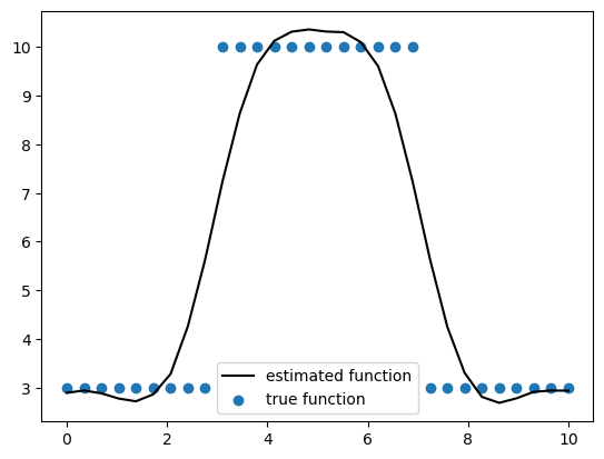
如上图所示,指数二次协方差函数过于缓慢,无法捕捉到突变,同时也由于过于平滑而过度偏离了变化。
结论#
案例研究向我们展示了如何利用HSGP将空间信息纳入我们的估计中。具体来说,我们了解了如何验证我们的模型规范,生成样本外估计,以及如何利用整个后验分布进行决策。
参考资料#
水印#
%load_ext watermark
%watermark -n -u -v -iv -w -p xarray
Last updated: Wed Aug 28 2024

Python implementation: CPython
Python version       : 3.12.4
IPython version      : 8.26.0

xarray: 2024.7.0

arviz      : 0.19.0
pandas     : 2.2.2
folium     : 0.17.0
mapclassify: 2.8.0
numpy      : 1.26.4
pymc       : 5.16.2
matplotlib : 3.9.1
rasterio   : 1.3.10
pytensor   : 2.25.2
geopandas  : 1.0.1

Watermark: 2.4.3
许可证声明#
本示例库中的所有笔记本均在MIT许可证下提供,该许可证允许修改和重新分发,前提是保留版权和许可证声明。
引用 PyMC 示例#
要引用此笔记本,请使用Zenodo为pymc-examples仓库提供的DOI。
重要
许多笔记本是从其他来源改编的:博客、书籍……在这种情况下,您应该引用原始来源。
同时记得引用代码中使用的相关库。
这是一个BibTeX的引用模板:
@incollection{citekey,
  author    = "<notebook authors, see above>",
  title     = "<notebook title>",
  editor    = "PyMC Team",
  booktitle = "PyMC examples",
  doi       = "10.5281/zenodo.5654871"
}
渲染后可能看起来像: