


贝叶斯生存分析#
生存分析研究事件发生时间分布。其应用涵盖医学、生物学、工程学和社会科学等多个领域。本教程展示了如何使用PyMC在Python中拟合和分析贝叶斯生存模型。
我们通过分析来自R的HSAUR包中的乳房切除术数据集来说明这些概念。
import arviz as az
import numpy as np
import pandas as pd
import pymc as pm
import pytensor

from matplotlib import pyplot as plt
from pymc.distributions.timeseries import GaussianRandomWalk
from pytensor import tensor as T

print(f"Running on PyMC v{pm.__version__}")
Running on PyMC v5.0.1+42.g99dd7158
RANDOM_SEED = 8927
rng = np.random.default_rng(RANDOM_SEED)
az.style.use("arviz-darkgrid")
try:
    df = pd.read_csv("../data/mastectomy.csv")
except FileNotFoundError:
    df = pd.read_csv(pm.get_data("mastectomy.csv"))

df.event = df.event.astype(np.int64)
df.metastasized = (df.metastasized == "yes").astype(np.int64)
n_patients = df.shape[0]
patients = np.arange(n_patients)
df.head()
| time | event | metastasized | |
|---|---|---|---|
| 0 | 23 | 1 | 0 |
| 1 | 47 | 1 | 0 |
| 2 | 69 | 1 | 0 |
| 3 | 70 | 0 | 0 |
| 4 | 100 | 0 | 0 |
n_patients
44
每一行代表一位接受乳房切除术并被诊断为乳腺癌的女性的观察数据。列 time 表示手术后观察该女性的时间(以月为单位)。列 event 表示在该观察期间该女性是否死亡。列 metastasized 表示癌症在手术前是否已 转移。
本教程分析了乳房切除术后生存时间与癌症是否转移之间的关系。
生存分析速成课程#
首先我们介绍一点(非常少)的理论。 如果随机变量 \(T\) 是我们研究的事件发生的时间,生存分析主要关注生存函数
其中 \(F\) 是 CDF 的 \(T\)。 从数学上讲,用 风险率 \(\lambda(t)\) 来表示生存函数是很方便的。 风险率是在时间 \(t\) 时事件发生的瞬时概率,假设它尚未发生。 也就是说,
求解此微分方程以得到生存函数表明
这种生存函数的表示方法表明了累积危险函数
是生存分析中的一个重要量,因为我们可以简洁地写成 \(S(t) = \exp(-\Lambda(t)).\)。
生存分析中一个重要但微妙的点是删失。尽管我们感兴趣的估计量是手术与死亡之间的时间,但我们并未观察到每个受试者的死亡。在我们进行分析的时间点,我们的一些受试者幸运地仍然活着。在我们的乳房切除术研究案例中,df.event 如果观察到了受试者的死亡(观察未被删失)则为1,如果未观察到死亡(观察被删失)则为0。
df.event.mean()
0.5909090909090909
我们观察到的数据中,超过40%的数据被截断。我们在下方可视化了观察到的持续时间,并标示了哪些观察结果被截断。
fig, ax = plt.subplots(figsize=(8, 6))

ax.hlines(
    patients[df.event.values == 0], 0, df[df.event.values == 0].time, color="C3", label="Censored"
)

ax.hlines(
    patients[df.event.values == 1], 0, df[df.event.values == 1].time, color="C7", label="Uncensored"
)

ax.scatter(
    df[df.metastasized.values == 1].time,
    patients[df.metastasized.values == 1],
    color="k",
    zorder=10,
    label="Metastasized",
)

ax.set_xlim(left=0)
ax.set_xlabel("Months since mastectomy")
ax.set_yticks([])
ax.set_ylabel("Subject")

ax.set_ylim(-0.25, n_patients + 0.25)

ax.legend(loc="center right");
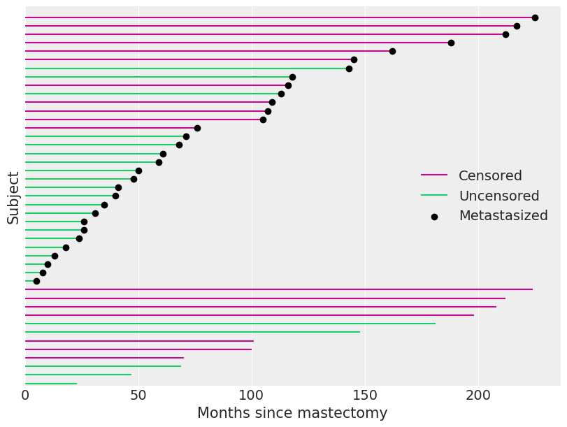
当一个观测值被删失时(df.event为零),df.time不是该受试者的生存时间。 我们只能从这种删失的观测中得出结论,即受试者的真实生存时间超过了df.time。
本教程的目的已经足够基本的生存分析理论;如需更广泛的介绍,请参阅Aalen等人。^[Aalen, Odd, Ornulf Borgan, 和 Hakon Gjessing. 生存和事件历史分析:过程观点。Springer Science & Business Media, 2008.]
贝叶斯比例风险模型#
生存分析中最基本的两个估计量是生存函数的Kaplan-Meier估计量和累积危险函数的Nelson-Aalen估计量。然而,由于我们想要了解转移对生存时间的影响,风险回归模型更为合适。也许最常用的风险回归模型是Cox的比例风险模型。在这个模型中,如果我们有协变量\(\mathbf{x}\)和回归系数\(\beta\),危险率被建模为
这里 \(\lambda_0(t)\) 是基准风险,它与协变量 \(\mathbf{x}\) 无关。在这个例子中,协变量是一维向量 df.metastasized。
与许多回归情况不同,\(\mathbf{x}\) 不应包含对应于截距的常数项。如果 \(\mathbf{x}\) 包含对应于截距的常数项,模型将变得不可识别。为了说明这种不可识别性,假设
如果 \(\tilde{\beta}_0 = \beta_0 + \delta\) 和 \(\tilde{\lambda}_0(t) = \lambda_0(t) \exp(-\delta)\),那么 \(\lambda(t) = \tilde{\lambda}_0(t) \exp(\tilde{\beta}_0 + \mathbf{x} \beta)\) 也同样成立,使得带有 \(\beta_0\) 的模型不可识别。
为了使用Cox模型进行贝叶斯推断,我们必须对\(\beta\)和\(\lambda_0(t)\)指定先验。我们对\(\beta\)放置一个正态先验,\(\beta \sim N(\mu_{\beta}, \sigma_{\beta}^2),\)其中\(\mu_{\beta} \sim N(0, 10^2)\)和\(\sigma_{\beta} \sim U(0, 10)\)。
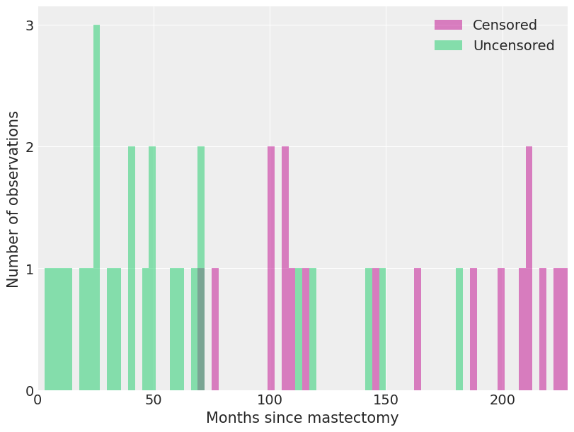
关于\(\lambda_0(t)\)的合适先验并不明显。我们选择了一个半参数先验,其中\(\lambda_0(t)\)是一个分段常数函数。这个先验要求我们将所考虑的时间范围划分为具有端点\(0 \leq s_1 < s_2 < \cdots < s_N\)的区间。在这个划分下,如果\(s_j \leq t < s_{j + 1}\),则\(\lambda_0 (t) = \lambda_j\)。由于\(\lambda_0(t)\)被限制为这种形式,我们只需要为\(N - 1\)个值\(\lambda_j\)选择先验。我们使用独立的模糊先验\(\lambda_j \sim \operatorname{Gamma}(10^{-2}, 10^{-2})\)。对于我们的乳房切除术示例,我们将每个区间设为三个月长。
我们观察到死亡和截尾观测在这些区间内的分布情况。
fig, ax = plt.subplots(figsize=(8, 6))

ax.hist(
    df[df.event == 0].time.values,
    bins=interval_bounds,
    lw=0,
    color="C3",
    alpha=0.5,
    label="Censored",
)

ax.hist(
    df[df.event == 1].time.values,
    bins=interval_bounds,
    lw=0,
    color="C7",
    alpha=0.5,
    label="Uncensored",
)

ax.set_xlim(0, interval_bounds[-1])
ax.set_xlabel("Months since mastectomy")

ax.set_yticks([0, 1, 2, 3])
ax.set_ylabel("Number of observations")

ax.legend();
在选择了\(\beta\)和\(\lambda_0(t)\)的先验分布后,我们现在展示如何使用pymc进行MCMC模拟来拟合模型。关键的观察是,分段常数比例风险模型与泊松回归模型密切相关。(这些模型并不完全相同,但它们的似然函数相差一个仅依赖于观测数据而不依赖于参数\(\beta\)和\(\lambda_j\)的因子。有关详细信息,请参阅Germán Rodríguez的WWS 509课程笔记。)
我们根据第\(i\)个受试者是否在第\(j\)个区间内死亡来定义指示变量,
我们还定义 \(t_{i, j}\) 为第 \(i\) 个受试者在第 \(j\) 个区间内处于风险中的时间。
exposure = np.greater_equal.outer(df.time.to_numpy(), interval_bounds[:-1]) * interval_length
exposure[patients, last_period] = df.time - interval_bounds[last_period]
最后,将第\(i\)个个体在第\(j\)个区间内所承担的风险表示为\(\lambda_{i, j} = \lambda_j \exp(\mathbf{x}_i \beta)\)。
我们可以用均值为 \(t_{i, j}\ \lambda_{i, j}\) 的泊松随机变量来近似 \(d_{i, j}\)。这个近似导致了以下 pymc 模型。
coords = {"intervals": intervals}

with pm.Model(coords=coords) as model:
    lambda0 = pm.Gamma("lambda0", 0.01, 0.01, dims="intervals")

    beta = pm.Normal("beta", 0, sigma=1000)

    lambda_ = pm.Deterministic("lambda_", T.outer(T.exp(beta * df.metastasized), lambda0))
    mu = pm.Deterministic("mu", exposure * lambda_)

    obs = pm.Poisson("obs", mu, observed=death)
我们现在从模型中进行采样。
n_samples = 1000
n_tune = 1000
with model:
    idata = pm.sample(
        n_samples,
        tune=n_tune,
        target_accept=0.99,
        random_seed=RANDOM_SEED,
    )
Auto-assigning NUTS sampler...
Initializing NUTS using jitter+adapt_diag...
Multiprocess sampling (4 chains in 4 jobs)
NUTS: [lambda0, beta]
Sampling 4 chains for 1_000 tune and 1_000 draw iterations (4_000 + 4_000 draws total) took 304 seconds.
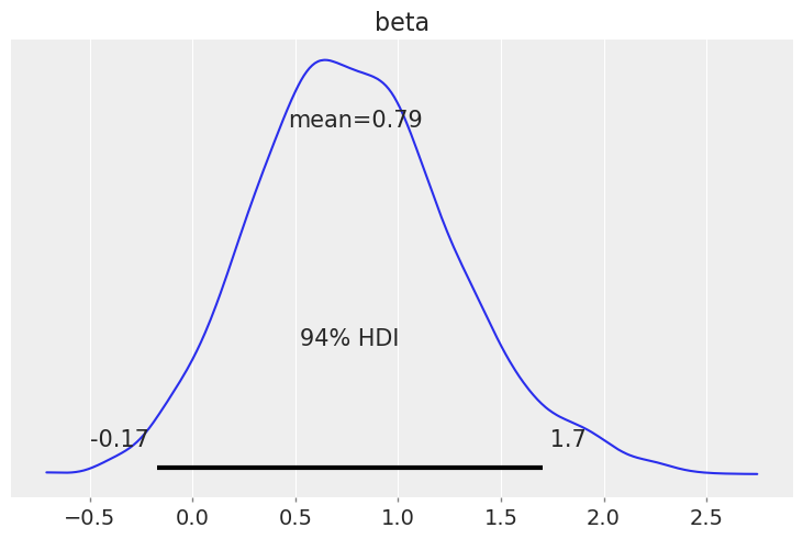
我们看到,癌症已经转移的患者的危险率大约是癌症未转移患者的1.5倍。
np.exp(idata.posterior["beta"]).mean()
<xarray.DataArray 'beta' ()>
array(2.51161491)
az.plot_posterior(idata, var_names=["beta"]);
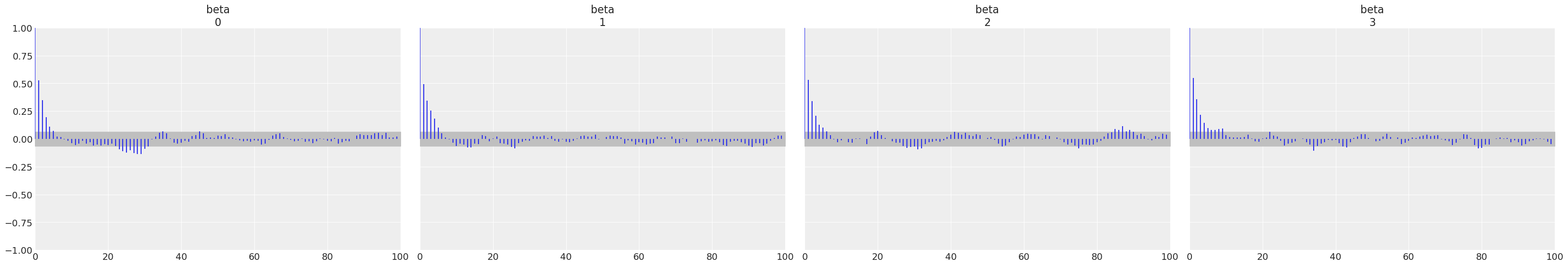
az.plot_autocorr(idata, var_names=["beta"]);
我们现在研究转移对累积危险函数和生存函数的影响。
base_hazard = idata.posterior["lambda0"]
met_hazard = idata.posterior["lambda0"] * np.exp(idata.posterior["beta"])
def cum_hazard(hazard):
    return (interval_length * hazard).cumsum(axis=-1)


def survival(hazard):
    return np.exp(-cum_hazard(hazard))


def get_mean(trace):
    return trace.mean(("chain", "draw"))
fig, (hazard_ax, surv_ax) = plt.subplots(ncols=2, sharex=True, sharey=False, figsize=(16, 6))

az.plot_hdi(
    interval_bounds[:-1],
    cum_hazard(base_hazard),
    ax=hazard_ax,
    smooth=False,
    color="C0",
    fill_kwargs={"label": "Had not metastasized"},
)
az.plot_hdi(
    interval_bounds[:-1],
    cum_hazard(met_hazard),
    ax=hazard_ax,
    smooth=False,
    color="C1",
    fill_kwargs={"label": "Metastasized"},
)

hazard_ax.plot(interval_bounds[:-1], get_mean(cum_hazard(base_hazard)), color="darkblue")
hazard_ax.plot(interval_bounds[:-1], get_mean(cum_hazard(met_hazard)), color="maroon")

hazard_ax.set_xlim(0, df.time.max())
hazard_ax.set_xlabel("Months since mastectomy")
hazard_ax.set_ylabel(r"Cumulative hazard $\Lambda(t)$")
hazard_ax.legend(loc=2)

az.plot_hdi(interval_bounds[:-1], survival(base_hazard), ax=surv_ax, smooth=False, color="C0")
az.plot_hdi(interval_bounds[:-1], survival(met_hazard), ax=surv_ax, smooth=False, color="C1")

surv_ax.plot(interval_bounds[:-1], get_mean(survival(base_hazard)), color="darkblue")
surv_ax.plot(interval_bounds[:-1], get_mean(survival(met_hazard)), color="maroon")

surv_ax.set_xlim(0, df.time.max())
surv_ax.set_xlabel("Months since mastectomy")
surv_ax.set_ylabel("Survival function $S(t)$")

fig.suptitle("Bayesian survival model");
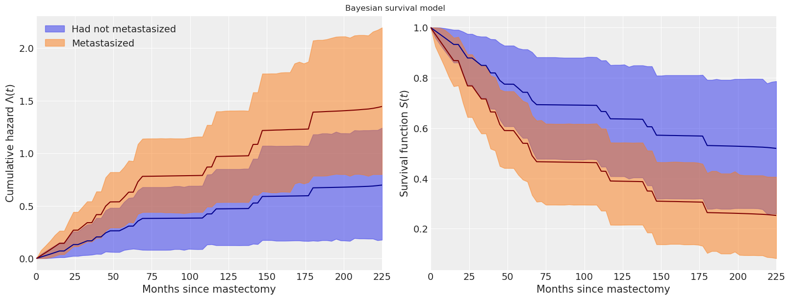
我们看到,转移性患者的累积风险在最初(大约七十个月)增加得更快,之后它与基线累积风险大致平行增加。
这些图还显示了每个函数的逐点95%高后验密度区间。使用pymc进行贝叶斯模型拟合的一个显著优势是,它能够自然地量化我们估计中的不确定性。
时间变化效应#
我们构建的模型的另一个优势是其灵活性。从上面的图表中,我们可以合理地相信,由于转移导致的额外风险随时间变化;似乎有理由认为,癌症在乳房切除术后立即增加了风险率,但随着时间的推移,转移导致的风险会降低。我们可以在模型中通过允许回归系数随时间变化来适应这一机制。在时间变化的系数模型中,如果 \(s_j \leq t < s_{j + 1}\),我们让 \(\lambda(t) = \lambda_j \exp(\mathbf{x} \beta_j).\) 回归系数的序列 \(\beta_1, \beta_2, \ldots, \beta_{N - 1}\) 形成一个正态随机游走,其中 \(\beta_1 \sim N(0, 1)\),\(\beta_j\ |\ \beta_{j - 1} \sim N(\beta_{j - 1}, 1)\)。
我们在pymc中实现此模型,如下所示。
coords = {"intervals": intervals}

with pm.Model(coords=coords) as time_varying_model:
    lambda0 = pm.Gamma("lambda0", 0.01, 0.01, dims="intervals")
    beta = GaussianRandomWalk("beta", init_dist=pm.Normal.dist(), sigma=1.0, dims="intervals")

    lambda_ = pm.Deterministic("h", lambda0 * T.exp(T.outer(T.constant(df.metastasized), beta)))
    mu = pm.Deterministic("mu", exposure * lambda_)

    obs = pm.Poisson("obs", mu, observed=death)
我们从该模型中进行采样。
with time_varying_model:
    time_varying_idata = pm.sample(
        n_samples,
        tune=n_tune,
        return_inferencedata=True,
        target_accept=0.99,
        random_seed=RANDOM_SEED,
    )
/home/cfonnesbeck/GitHub/pymc/pymc/logprob/joint_logprob.py:167: UserWarning: Found a random variable that was neither among the observations nor the conditioned variables: [normal_rv{0, (0, 0), floatX, False}.0, normal_rv{0, (0, 0), floatX, False}.out]
  warnings.warn(
/home/cfonnesbeck/GitHub/pymc/pymc/logprob/joint_logprob.py:167: UserWarning: Found a random variable that was neither among the observations nor the conditioned variables: [normal_rv{0, (0, 0), floatX, False}.0, normal_rv{0, (0, 0), floatX, False}.out]
  warnings.warn(
Auto-assigning NUTS sampler...
Initializing NUTS using jitter+adapt_diag...
/home/cfonnesbeck/GitHub/pymc/pymc/logprob/joint_logprob.py:167: UserWarning: Found a random variable that was neither among the observations nor the conditioned variables: [normal_rv{0, (0, 0), floatX, False}.0, normal_rv{0, (0, 0), floatX, False}.out]
  warnings.warn(
/home/cfonnesbeck/GitHub/pymc/pymc/logprob/joint_logprob.py:167: UserWarning: Found a random variable that was neither among the observations nor the conditioned variables: [normal_rv{0, (0, 0), floatX, False}.0, normal_rv{0, (0, 0), floatX, False}.out]
  warnings.warn(
/home/cfonnesbeck/GitHub/pymc/pymc/logprob/joint_logprob.py:167: UserWarning: Found a random variable that was neither among the observations nor the conditioned variables: [normal_rv{0, (0, 0), floatX, False}.0, normal_rv{0, (0, 0), floatX, False}.out]
  warnings.warn(
/home/cfonnesbeck/GitHub/pymc/pymc/logprob/joint_logprob.py:167: UserWarning: Found a random variable that was neither among the observations nor the conditioned variables: [normal_rv{0, (0, 0), floatX, False}.0, normal_rv{0, (0, 0), floatX, False}.out]
  warnings.warn(
/home/cfonnesbeck/GitHub/pymc/pymc/logprob/joint_logprob.py:167: UserWarning: Found a random variable that was neither among the observations nor the conditioned variables: [normal_rv{0, (0, 0), floatX, False}.0, normal_rv{0, (0, 0), floatX, False}.out]
  warnings.warn(
/home/cfonnesbeck/GitHub/pymc/pymc/logprob/joint_logprob.py:167: UserWarning: Found a random variable that was neither among the observations nor the conditioned variables: [normal_rv{0, (0, 0), floatX, False}.0, normal_rv{0, (0, 0), floatX, False}.out]
  warnings.warn(
/home/cfonnesbeck/GitHub/pymc/pymc/logprob/joint_logprob.py:167: UserWarning: Found a random variable that was neither among the observations nor the conditioned variables: [normal_rv{0, (0, 0), floatX, False}.0, normal_rv{0, (0, 0), floatX, False}.out]
  warnings.warn(
/home/cfonnesbeck/GitHub/pymc/pymc/logprob/joint_logprob.py:167: UserWarning: Found a random variable that was neither among the observations nor the conditioned variables: [normal_rv{0, (0, 0), floatX, False}.0, normal_rv{0, (0, 0), floatX, False}.out]
  warnings.warn(
/home/cfonnesbeck/GitHub/pymc/pymc/logprob/joint_logprob.py:167: UserWarning: Found a random variable that was neither among the observations nor the conditioned variables: [normal_rv{0, (0, 0), floatX, False}.0, normal_rv{0, (0, 0), floatX, False}.out]
  warnings.warn(
Multiprocess sampling (4 chains in 4 jobs)
NUTS: [lambda0, beta]
Sampling 4 chains for 1_000 tune and 1_000 draw iterations (4_000 + 4_000 draws total) took 536 seconds.
az.plot_forest(time_varying_idata, var_names=["beta"]);
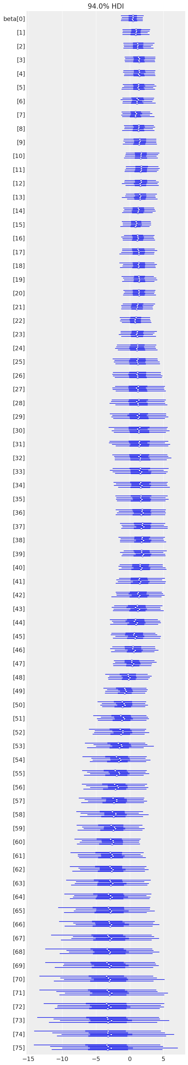
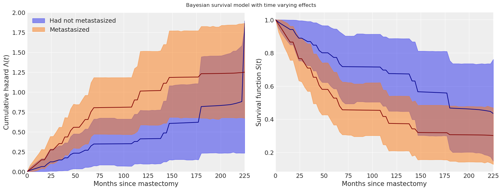
我们从下面的时间序列图中看到,\(\beta_j\) 最初 \(\beta_j > 0\),表明由于转移导致的危险率升高,但随着时间的推移,这种风险最终会下降,\(\beta_j < 0\)。
fig, ax = plt.subplots(figsize=(8, 6))

beta_eti = time_varying_idata.posterior["beta"].quantile((0.025, 0.975), dim=("chain", "draw"))
beta_eti_low = beta_eti.sel(quantile=0.025)
beta_eti_high = beta_eti.sel(quantile=0.975)

ax.fill_between(interval_bounds[:-1], beta_eti_low, beta_eti_high, color="C0", alpha=0.25)

beta_hat = time_varying_idata.posterior["beta"].mean(("chain", "draw"))

ax.step(interval_bounds[:-1], beta_hat, color="C0")

ax.scatter(
    interval_bounds[last_period[(df.event.values == 1) & (df.metastasized == 1)]],
    beta_hat.isel(intervals=last_period[(df.event.values == 1) & (df.metastasized == 1)]),
    color="C1",
    zorder=10,
    label="Died, cancer metastasized",
)

ax.scatter(
    interval_bounds[last_period[(df.event.values == 0) & (df.metastasized == 1)]],
    beta_hat.isel(intervals=last_period[(df.event.values == 0) & (df.metastasized == 1)]),
    color="C0",
    zorder=10,
    label="Censored, cancer metastasized",
)

ax.set_xlim(0, df.time.max())
ax.set_xlabel("Months since mastectomy")
ax.set_ylabel(r"$\beta_j$")
ax.legend();
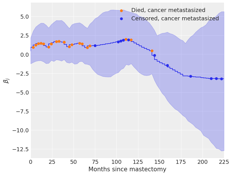
系数 \(\beta_j\) 在大约一百个月后开始迅速下降,这似乎是合理的,因为在这项研究中,只有十二名癌症已经转移的受试者中有三人活过了这个时间点。
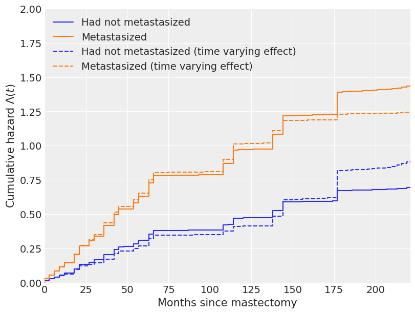
由于时间变化效应,我们对累积危险函数和生存函数估计的变化在以下图中也相当明显。
tv_base_hazard = time_varying_idata.posterior["lambda0"]
tv_met_hazard = time_varying_idata.posterior["lambda0"] * np.exp(
    time_varying_idata.posterior["beta"]
)
fig, ax = plt.subplots(figsize=(8, 6))

ax.step(
    interval_bounds[:-1],
    cum_hazard(base_hazard.mean(("chain", "draw"))),
    color="C0",
    label="Had not metastasized",
)

ax.step(
    interval_bounds[:-1],
    cum_hazard(met_hazard.mean(("chain", "draw"))),
    color="C1",
    label="Metastasized",
)

ax.step(
    interval_bounds[:-1],
    cum_hazard(tv_base_hazard.mean(("chain", "draw"))),
    color="C0",
    linestyle="--",
    label="Had not metastasized (time varying effect)",
)

ax.step(
    interval_bounds[:-1],
    cum_hazard(tv_met_hazard.mean(dim=("chain", "draw"))),
    color="C1",
    linestyle="--",
    label="Metastasized (time varying effect)",
)

ax.set_xlim(0, df.time.max() - 4)
ax.set_xlabel("Months since mastectomy")
ax.set_ylim(0, 2)
ax.set_ylabel(r"Cumulative hazard $\Lambda(t)$")
ax.legend(loc=2);
fig, (hazard_ax, surv_ax) = plt.subplots(ncols=2, sharex=True, sharey=False, figsize=(16, 6))

az.plot_hdi(
    interval_bounds[:-1],
    cum_hazard(tv_base_hazard),
    ax=hazard_ax,
    color="C0",
    smooth=False,
    fill_kwargs={"label": "Had not metastasized"},
)

az.plot_hdi(
    interval_bounds[:-1],
    cum_hazard(tv_met_hazard),
    ax=hazard_ax,
    smooth=False,
    color="C1",
    fill_kwargs={"label": "Metastasized"},
)

hazard_ax.plot(interval_bounds[:-1], get_mean(cum_hazard(tv_base_hazard)), color="darkblue")
hazard_ax.plot(interval_bounds[:-1], get_mean(cum_hazard(tv_met_hazard)), color="maroon")

hazard_ax.set_xlim(0, df.time.max())
hazard_ax.set_xlabel("Months since mastectomy")
hazard_ax.set_ylim(0, 2)
hazard_ax.set_ylabel(r"Cumulative hazard $\Lambda(t)$")
hazard_ax.legend(loc=2)

az.plot_hdi(interval_bounds[:-1], survival(tv_base_hazard), ax=surv_ax, smooth=False, color="C0")
az.plot_hdi(interval_bounds[:-1], survival(tv_met_hazard), ax=surv_ax, smooth=False, color="C1")

surv_ax.plot(interval_bounds[:-1], get_mean(survival(tv_base_hazard)), color="darkblue")
surv_ax.plot(interval_bounds[:-1], get_mean(survival(tv_met_hazard)), color="maroon")

surv_ax.set_xlim(0, df.time.max())
surv_ax.set_xlabel("Months since mastectomy")
surv_ax.set_ylabel("Survival function $S(t)$")
fig.suptitle("Bayesian survival model with time varying effects");
我们实际上只是触及了生存分析和贝叶斯生存分析方法的表面。关于贝叶斯生存分析的更多信息可以在Ibrahim等人(2005年)中找到。(例如,我们可能希望在原始或时间变化模型中考虑个体脆弱性。)
许可证声明#
本示例库中的所有笔记本均在MIT许可证下提供,该许可证允许修改和重新分发,前提是保留版权和许可证声明。
引用 PyMC 示例#
要引用此笔记本,请使用Zenodo为pymc-examples仓库提供的DOI。
重要
许多笔记本是从其他来源改编的:博客、书籍……在这种情况下,您应该引用原始来源。
同时记得引用代码中使用的相关库。
这是一个BibTeX的引用模板:
@incollection{citekey,
  author    = "<notebook authors, see above>",
  title     = "<notebook title>",
  editor    = "PyMC Team",
  booktitle = "PyMC examples",
  doi       = "10.5281/zenodo.5654871"
}
渲染后可能看起来像: