重新参数化Weibull加速失效时间模型#

import arviz as az
import numpy as np
import pymc as pm
import pytensor.tensor as pt
import statsmodels.api as sm

print(f"Running on PyMC v{pm.__version__}")

Running on PyMC v5.0.1+42.g99dd7158

%config InlineBackend.figure_format = 'retina'
RANDOM_SEED = 8927
np.random.seed(RANDOM_SEED)
az.style.use("arviz-darkgrid")

数据集#

之前的关于贝叶斯参数生存分析的示例笔记本介绍了两种不同的加速失效时间（AFT）模型：Weibull和线性对数模型。在本笔记本中，我们介绍了Weibull AFT模型的三种不同参数化方法。

我们将使用的数据集是 flchain R 数据集，该数据集来自一项医学研究，研究血清游离轻链 (FLC) 对寿命的影响。通过运行以下命令阅读数据的完整文档：

print(sm.datasets.get_rdataset(package='survival', dataname='flchain').__doc__)。

# Fetch and clean data
data = (
    sm.datasets.get_rdataset(package="survival", dataname="flchain")
    .data.sample(500)  # Limit ourselves to 500 observations
    .reset_index(drop=True)
)

y = data.futime.values
censored = ~data["death"].values.astype(bool)

y[:5]

array([ 975, 2272,  138, 4262, 4928])

censored[:5]

array([False,  True, False,  True,  True])

使用 `pm.Potential`#

我们在对截尾数据进行建模时遇到了一个独特的问题。严格来说，我们没有任何关于截尾值的数据：我们只知道被截尾的数量。我们如何将这些信息纳入我们的模型中？

一种方法是利用pm.Potential。PyMC2 文档很好地解释了它的用法。本质上，声明pm.Potential('x', logp)会将logp添加到模型的对数似然中。

参数化 1#

这种参数化是威布尔生存函数的一种直观、直接的参数化方法。这可能是人们首先想到的参数化方法。

def weibull_lccdf(x, alpha, beta):
    """Log complementary cdf of Weibull distribution."""
    return -((x / beta) ** alpha)

with pm.Model() as model_1:
    alpha_sd = 10.0

    mu = pm.Normal("mu", mu=0, sigma=100)
    alpha_raw = pm.Normal("a0", mu=0, sigma=0.1)
    alpha = pm.Deterministic("alpha", pt.exp(alpha_sd * alpha_raw))
    beta = pm.Deterministic("beta", pt.exp(mu / alpha))

    y_obs = pm.Weibull("y_obs", alpha=alpha, beta=beta, observed=y[~censored])
    y_cens = pm.Potential("y_cens", weibull_lccdf(y[censored], alpha, beta))

with model_1:
    # Change init to avoid divergences
    data_1 = pm.sample(target_accept=0.9, init="adapt_diag")

Auto-assigning NUTS sampler...
Initializing NUTS using adapt_diag...
Multiprocess sampling (4 chains in 4 jobs)
NUTS: [mu, a0]

100.00% [8000/8000 00:09<00:00 Sampling 4 chains, 0 divergences]

Sampling 4 chains for 1_000 tune and 1_000 draw iterations (4_000 + 4_000 draws total) took 10 seconds.

az.plot_trace(data_1, var_names=["alpha", "beta"])

array([[<AxesSubplot: title={'center': 'alpha'}>,
        <AxesSubplot: title={'center': 'alpha'}>],
       [<AxesSubplot: title={'center': 'beta'}>,
        <AxesSubplot: title={'center': 'beta'}>]], dtype=object)

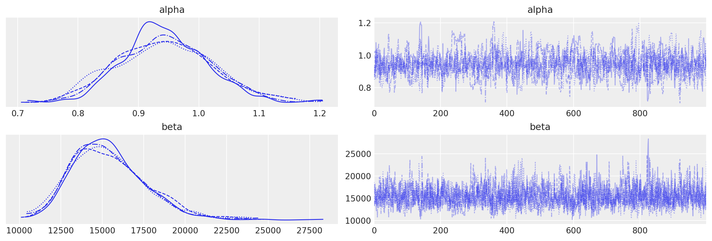
../_images/f034caeb8837a0882fdcfee00061523154796389848e8b2f1a856fe9a4191854.png

az.summary(data_1, var_names=["alpha", "beta"], round_to=2)

	mean	sd	hdi_3%	hdi_97%	mcse_mean	mcse_sd	ess_bulk	ess_tail	r_hat
alpha	0.94	0.08	0.80	1.08	0.00	0.00	735.35	701.64	1.01
beta	15386.70	2269.14	11442.57	19562.58	65.38	46.48	1228.87	1682.03	1.00

参数化 2#

需要注意的是，令人困惑的是，alpha 现在被称为 r，而 alpha 表示一个先验；我们保持这种符号以忠实于Stan中的原始实现。在这种参数化中，我们仍然对相同的参数 alpha（现在是 r）和 beta 进行建模。

更多信息，请参阅这个 Stan 示例模型和相应的文档。

with pm.Model() as model_2:
    alpha = pm.Normal("alpha", mu=0, sigma=10)
    r = pm.Gamma("r", alpha=1, beta=0.001, testval=0.25)
    beta = pm.Deterministic("beta", pt.exp(-alpha / r))

    y_obs = pm.Weibull("y_obs", alpha=r, beta=beta, observed=y[~censored])
    y_cens = pm.Potential("y_cens", weibull_lccdf(y[censored], r, beta))

/tmp/ipykernel_915/3602845657.py:3: FutureWarning: The `testval` argument is deprecated; use `initval`.
  r = pm.Gamma("r", alpha=1, beta=0.001, testval=0.25)

with model_2:
    # Increase target_accept to avoid divergences
    data_2 = pm.sample(target_accept=0.9)

Auto-assigning NUTS sampler...
Initializing NUTS using jitter+adapt_diag...
Multiprocess sampling (4 chains in 4 jobs)
NUTS: [alpha, r]

100.00% [8000/8000 00:10<00:00 Sampling 4 chains, 0 divergences]

Sampling 4 chains for 1_000 tune and 1_000 draw iterations (4_000 + 4_000 draws total) took 10 seconds.

az.plot_trace(data_2, var_names=["r", "beta"])

array([[<AxesSubplot: title={'center': 'r'}>,
        <AxesSubplot: title={'center': 'r'}>],
       [<AxesSubplot: title={'center': 'beta'}>,
        <AxesSubplot: title={'center': 'beta'}>]], dtype=object)

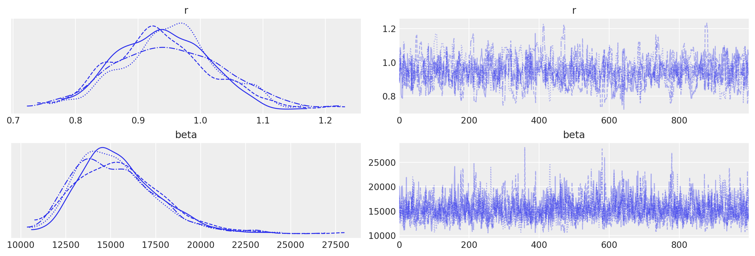
../_images/fb168cb151323b9ca1c6733a33edfa07fa0c90a8a25a80beaed731d6b65636b1.png

az.summary(data_2, var_names=["r", "beta"], round_to=2)

	mean	sd	hdi_3%	hdi_97%	mcse_mean	mcse_sd	ess_bulk	ess_tail	r_hat
r	0.94	0.08	0.80	1.10	0.0	0.00	702.52	671.31	1.01
beta	15377.49	2313.49	11423.58	19710.63	65.1	46.47	1284.63	1696.35	1.00

参数化 3#

在这个参数化中，我们使用Gumbel分布来建模对数线性误差分布，而不是直接建模生存函数。更多信息，请参见这篇博客文章。

logtime = np.log(y)


def gumbel_sf(y, mu, sigma):
    """Gumbel survival function."""
    return 1.0 - pt.exp(-pt.exp(-(y - mu) / sigma))

with pm.Model() as model_3:
    s = pm.HalfNormal("s", tau=5.0)
    gamma = pm.Normal("gamma", mu=0, sigma=5)

    y_obs = pm.Gumbel("y_obs", mu=gamma, beta=s, observed=logtime[~censored])
    y_cens = pm.Potential("y_cens", gumbel_sf(y=logtime[censored], mu=gamma, sigma=s))

with model_3:
    # Change init to avoid divergences
    data_3 = pm.sample(init="adapt_diag")

Auto-assigning NUTS sampler...
Initializing NUTS using adapt_diag...
Multiprocess sampling (4 chains in 4 jobs)
NUTS: [s, gamma]

100.00% [8000/8000 00:03<00:00 Sampling 4 chains, 0 divergences]

Sampling 4 chains for 1_000 tune and 1_000 draw iterations (4_000 + 4_000 draws total) took 4 seconds.

az.plot_trace(data_3)

array([[<AxesSubplot: title={'center': 'gamma'}>,
        <AxesSubplot: title={'center': 'gamma'}>],
       [<AxesSubplot: title={'center': 's'}>,
        <AxesSubplot: title={'center': 's'}>]], dtype=object)

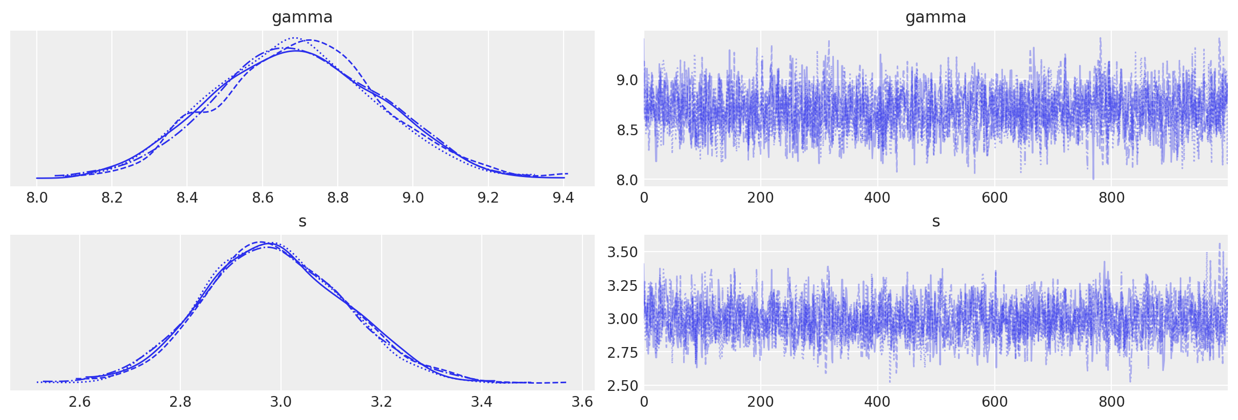
../_images/5e8d109c7618f5ea4e21d87235f664604b8be8a6567ab819166a070babe4a8d7.png

az.summary(data_3, round_to=2)

	mean	sd	hdi_3%	hdi_97%	mcse_mean	mcse_sd	ess_bulk	ess_tail	r_hat
gamma	8.69	0.22	8.31	9.11	0.0	0.0	2233.04	2305.13	1.0
s	2.99	0.14	2.74	3.26	0.0	0.0	2067.28	2328.40	1.0

作者#

最初由 Junpeng Lao 于 2018 年 4 月 21 日整理。查看原始代码在此。
由 George Ho 于2018年7月15日创作并移植到Jupyter笔记本。
更新以兼容 PyMC v5，由 Chris Fonnesbeck 于 2023 年 1 月 16 日完成。

%load_ext watermark
%watermark -n -u -v -iv -w

Last updated: Tue Jan 17 2023

Python implementation: CPython
Python version       : 3.11.0
IPython version      : 8.8.0

arviz      : 0.14.0
numpy      : 1.24.1
pymc       : 5.0.1+42.g99dd7158
sys        : 3.11.0 | packaged by conda-forge | (main, Oct 25 2022, 06:24:40) [GCC 10.4.0]
pytensor   : 2.9.1
statsmodels: 0.13.5

Watermark: 2.3.1

许可证声明#

本示例库中的所有笔记本均在MIT许可证下提供，该许可证允许修改和重新分发，前提是保留版权和许可证声明。

引用 PyMC 示例#

要引用此笔记本，请使用Zenodo为pymc-examples仓库提供的DOI。

重要

许多笔记本是从其他来源改编的：博客、书籍……在这种情况下，您应该引用原始来源。

同时记得引用代码中使用的相关库。

这是一个BibTeX的引用模板：

@incollection{citekey,
  author    = "<notebook authors, see above>",
  title     = "<notebook title>",
  editor    = "PyMC Team",
  booktitle = "PyMC examples",
  doi       = "10.5281/zenodo.5654871"
}

渲染后可能看起来像：

分类

标签

重新参数化Weibull加速失效时间模型#

数据集#

使用 `pm.Potential`#

参数化 1#

参数化 2#

参数化 3#

作者#

许可证声明#

引用 PyMC 示例#

分类

标签

重新参数化Weibull加速失效时间模型#

数据集#

使用 pm.Potential#

参数化 1#

参数化 2#

参数化 3#

作者#

许可证声明#

引用 PyMC 示例#

使用 `pm.Potential`#