多元高斯随机游走

import arviz as az
import matplotlib.pyplot as plt
import numpy as np
import pymc as pm
import pytensor

from scipy.linalg import cholesky

%matplotlib inline

RANDOM_SEED = 8927
rng = np.random.default_rng(RANDOM_SEED)
az.style.use("arviz-darkgrid")

本笔记本展示了如何使用多元高斯随机游走（GRWs）对相关时间序列进行拟合。特别是，我们对时间序列数据进行贝叶斯回归，该回归依赖于基于GRWs的模型。

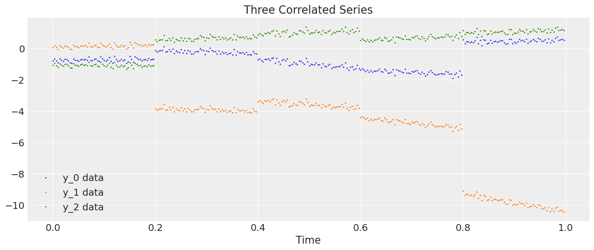
我们生成数据作为三维时间序列

()\[ \mathbf y = \alpha_{i[\mathbf t]} +\beta_{i[\mathbf t]} *\frac{\mathbf t}{300} +\xi_{\mathbf t},\quad \mathbf t = [0,1,...,299], \]

哪里

• \(i\mapsto\alpha_{i}\) 和 \(i\mapsto\beta_{i}\), \(i\in\{0,1,2,3,4\}\), 是两个三维高斯随机游走，分别对应两个相关矩阵 \(\Sigma_\alpha\) 和 \(\Sigma_\beta\)。

• 我们定义索引

  \[ i[t]= j\quad\text{对于}\quad t = 60j,60j+1,...,60j+59, \quad\text{并且}\quad j = 0,1,2,3,4, \]

• \(*\) 表示我们将 \(3\times300\) 矩阵的第 \(j\) 列与向量的第 \(j\) 个元素相乘，其中 \(j=0,1,...,299\)。

• \(\xi_{\mathbf t}\) 是一个 \(3\times300\) 的矩阵，其元素为独立同分布的正态分布 \(N(0,\sigma^2)\)。

因此，序列 \(\mathbf y\) 由于 GRW \(\alpha\) 在五个时刻发生变化，即步骤 \(0,60,120,180,240\)。同时，\(\mathbf y\) 在步骤 \(1,60,120,180,240\) 由于 GRW \(\beta\) 的增量而发生变化，并且在每一步由于 \(\beta\) 与 \(\mathbf t/300\) 的加权而发生变化。直观地说，我们有一个噪声（\(\xi\)）系统，在300个步骤的周期内受到五次冲击，但 \(\beta\) 冲击的影响在每一步逐渐变得更加显著。

数据生成

让我们生成并绘制数据。

D = 3  # Dimension of random walks
N = 300  # Number of steps
sections = 5  # Number of sections
period = N / sections  # Number steps in each section

Sigma_alpha = rng.standard_normal((D, D))
Sigma_alpha = Sigma_alpha.T.dot(Sigma_alpha)  # Construct covariance matrix for alpha
L_alpha = cholesky(Sigma_alpha, lower=True)  # Obtain its Cholesky decomposition

Sigma_beta = rng.standard_normal((D, D))
Sigma_beta = Sigma_beta.T.dot(Sigma_beta)  # Construct covariance matrix for beta
L_beta = cholesky(Sigma_beta, lower=True)  # Obtain its Cholesky decomposition

# Gaussian random walks:
alpha = np.cumsum(L_alpha.dot(rng.standard_normal((D, sections))), axis=1).T
beta = np.cumsum(L_beta.dot(rng.standard_normal((D, sections))), axis=1).T
t = np.arange(N)[:, None] / N
alpha = np.repeat(alpha, period, axis=0)
beta = np.repeat(beta, period, axis=0)
# Correlated series
sigma = 0.1
y = alpha + beta * t + sigma * rng.standard_normal((N, 1))

# Plot the correlated series
plt.figure(figsize=(12, 5))
plt.plot(t, y, ".", markersize=2, label=("y_0 data", "y_1 data", "y_2 data"))
plt.title("Three Correlated Series")
plt.xlabel("Time")
plt.legend()
plt.show();

模型

首先我们引入一个缩放类来重新缩放我们的数据和采样前的时间参数，然后将预测结果重新缩放以匹配未缩放的数据。

class Scaler:
    def __init__(self):
        mean_ = None
        std_ = None

    def transform(self, x):
        return (x - self.mean_) / self.std_

    def fit_transform(self, x):
        self.mean_ = x.mean(axis=0)
        self.std_ = x.std(axis=0)
        return self.transform(x)

    def inverse_transform(self, x):
        return x * self.std_ + self.mean_

我们现在在（）中构建回归模型，对GRWs \(\alpha\) 和 \(\beta\)，标准差 \(\sigma\) 以及Cholesky矩阵的超先验施加先验。我们使用LKJ先验 [Lewandowski 等人, 2009] 用于Cholesky矩阵（参见此链接 以获取文档，以及PyMC笔记本 /case_studies/LKJ 以获取一些使用示例。）

def inference(t, y, sections, n_samples=100):
    N, D = y.shape

    # Standardize y and t
    y_scaler = Scaler()
    t_scaler = Scaler()
    y = y_scaler.fit_transform(y)
    t = t_scaler.fit_transform(t)
    # Create a section index
    t_section = np.repeat(np.arange(sections), N / sections)

    # Create PyTensor equivalent
    t_t = pytensor.shared(np.repeat(t, D, axis=1))
    y_t = pytensor.shared(y)
    t_section_t = pytensor.shared(t_section)

    coords = {"y_": ["y_0", "y_1", "y_2"], "steps": np.arange(N)}
    with pm.Model(coords=coords) as model:
        # Hyperpriors on Cholesky matrices
        chol_alpha, *_ = pm.LKJCholeskyCov(
            "chol_cov_alpha", n=D, eta=2, sd_dist=pm.HalfCauchy.dist(2.5), compute_corr=True
        )
        chol_beta, *_ = pm.LKJCholeskyCov(
            "chol_cov_beta", n=D, eta=2, sd_dist=pm.HalfCauchy.dist(2.5), compute_corr=True
        )

        # Priors on Gaussian random walks
        alpha = pm.MvGaussianRandomWalk(
            "alpha", mu=np.zeros(D), chol=chol_alpha, shape=(sections, D)
        )
        beta = pm.MvGaussianRandomWalk("beta", mu=np.zeros(D), chol=chol_beta, shape=(sections, D))

        # Deterministic construction of the correlated random walk
        alpha_r = alpha[t_section_t]
        beta_r = beta[t_section_t]
        regression = alpha_r + beta_r * t_t

        # Prior on noise ξ
        sigma = pm.HalfNormal("sigma", 1.0)

        # Likelihood
        likelihood = pm.Normal("y", mu=regression, sigma=sigma, observed=y_t, dims=("steps", "y_"))

        # MCMC sampling
        trace = pm.sample(n_samples, tune=1000, chains=4, target_accept=0.9)

        # Posterior predictive sampling
        pm.sample_posterior_predictive(trace, extend_inferencedata=True)

    return trace, y_scaler, t_scaler, t_section

推理

我们现在从我们的模型中进行采样，并返回轨迹、空间和时间的缩放函数以及缩放后的时间索引。

trace, y_scaler, t_scaler, t_section = inference(t, y, sections)

/Users/cfonnesbeck/mambaforge/envs/pie/lib/python3.9/site-packages/pymc/distributions/timeseries.py:345: UserWarning: Initial distribution not specified, defaulting to `MvNormal.dist(0, I*100)`.You can specify an init_dist manually to suppress this warning.
  warnings.warn(
/Users/cfonnesbeck/mambaforge/envs/pie/lib/python3.9/site-packages/pymc/distributions/timeseries.py:345: UserWarning: Initial distribution not specified, defaulting to `MvNormal.dist(0, I*100)`.You can specify an init_dist manually to suppress this warning.
  warnings.warn(
Only 100 samples in chain.
/Users/cfonnesbeck/mambaforge/envs/pie/lib/python3.9/site-packages/pymc/logprob/joint_logprob.py:167: UserWarning: Found a random variable that was neither among the observations nor the conditioned variables: [multivariate_normal_rv{1, (1, 2), floatX, False}.0, multivariate_normal_rv{1, (1, 2), floatX, False}.out]
  warnings.warn(
/Users/cfonnesbeck/mambaforge/envs/pie/lib/python3.9/site-packages/pymc/logprob/joint_logprob.py:167: UserWarning: Found a random variable that was neither among the observations nor the conditioned variables: [multivariate_normal_rv{1, (1, 2), floatX, False}.0, multivariate_normal_rv{1, (1, 2), floatX, False}.out]
  warnings.warn(
/Users/cfonnesbeck/mambaforge/envs/pie/lib/python3.9/site-packages/pymc/logprob/joint_logprob.py:167: UserWarning: Found a random variable that was neither among the observations nor the conditioned variables: [multivariate_normal_rv{1, (1, 2), floatX, False}.0, multivariate_normal_rv{1, (1, 2), floatX, False}.out]
  warnings.warn(
/Users/cfonnesbeck/mambaforge/envs/pie/lib/python3.9/site-packages/pymc/logprob/joint_logprob.py:167: UserWarning: Found a random variable that was neither among the observations nor the conditioned variables: [multivariate_normal_rv{1, (1, 2), floatX, False}.0, multivariate_normal_rv{1, (1, 2), floatX, False}.out]
  warnings.warn(
/Users/cfonnesbeck/mambaforge/envs/pie/lib/python3.9/site-packages/multipledispatch/dispatcher.py:27: AmbiguityWarning: 
Ambiguities exist in dispatched function _unify

The following signatures may result in ambiguous behavior:
	[ConstrainedVar, Var, Mapping], [object, ConstrainedVar, Mapping]
	[object, ConstrainedVar, Mapping], [ConstrainedVar, object, Mapping]
	[object, ConstrainedVar, Mapping], [ConstrainedVar, Var, Mapping]
	[ConstrainedVar, object, Mapping], [object, ConstrainedVar, Mapping]


Consider making the following additions:

@dispatch(ConstrainedVar, ConstrainedVar, Mapping)
def _unify(...)

@dispatch(ConstrainedVar, ConstrainedVar, Mapping)
def _unify(...)

@dispatch(ConstrainedVar, ConstrainedVar, Mapping)
def _unify(...)

@dispatch(ConstrainedVar, ConstrainedVar, Mapping)
def _unify(...)
  warn(warning_text(dispatcher.name, ambiguities), AmbiguityWarning)
Auto-assigning NUTS sampler...
Initializing NUTS using jitter+adapt_diag...
/Users/cfonnesbeck/mambaforge/envs/pie/lib/python3.9/site-packages/pymc/logprob/joint_logprob.py:167: UserWarning: Found a random variable that was neither among the observations nor the conditioned variables: [multivariate_normal_rv{1, (1, 2), floatX, False}.0, multivariate_normal_rv{1, (1, 2), floatX, False}.out]
  warnings.warn(
/Users/cfonnesbeck/mambaforge/envs/pie/lib/python3.9/site-packages/pymc/logprob/joint_logprob.py:167: UserWarning: Found a random variable that was neither among the observations nor the conditioned variables: [multivariate_normal_rv{1, (1, 2), floatX, False}.0, multivariate_normal_rv{1, (1, 2), floatX, False}.out]
  warnings.warn(
/Users/cfonnesbeck/mambaforge/envs/pie/lib/python3.9/site-packages/pymc/logprob/joint_logprob.py:167: UserWarning: Found a random variable that was neither among the observations nor the conditioned variables: [multivariate_normal_rv{1, (1, 2), floatX, False}.0, multivariate_normal_rv{1, (1, 2), floatX, False}.out]
  warnings.warn(
/Users/cfonnesbeck/mambaforge/envs/pie/lib/python3.9/site-packages/pymc/logprob/joint_logprob.py:167: UserWarning: Found a random variable that was neither among the observations nor the conditioned variables: [multivariate_normal_rv{1, (1, 2), floatX, False}.0, multivariate_normal_rv{1, (1, 2), floatX, False}.out]
  warnings.warn(
/Users/cfonnesbeck/mambaforge/envs/pie/lib/python3.9/site-packages/pymc/logprob/joint_logprob.py:167: UserWarning: Found a random variable that was neither among the observations nor the conditioned variables: [multivariate_normal_rv{1, (1, 2), floatX, False}.0, multivariate_normal_rv{1, (1, 2), floatX, False}.out]
  warnings.warn(
/Users/cfonnesbeck/mambaforge/envs/pie/lib/python3.9/site-packages/pymc/logprob/joint_logprob.py:167: UserWarning: Found a random variable that was neither among the observations nor the conditioned variables: [multivariate_normal_rv{1, (1, 2), floatX, False}.0, multivariate_normal_rv{1, (1, 2), floatX, False}.out]
  warnings.warn(
/Users/cfonnesbeck/mambaforge/envs/pie/lib/python3.9/site-packages/pymc/logprob/joint_logprob.py:167: UserWarning: Found a random variable that was neither among the observations nor the conditioned variables: [multivariate_normal_rv{1, (1, 2), floatX, False}.0, multivariate_normal_rv{1, (1, 2), floatX, False}.out]
  warnings.warn(
/Users/cfonnesbeck/mambaforge/envs/pie/lib/python3.9/site-packages/pymc/logprob/joint_logprob.py:167: UserWarning: Found a random variable that was neither among the observations nor the conditioned variables: [multivariate_normal_rv{1, (1, 2), floatX, False}.0, multivariate_normal_rv{1, (1, 2), floatX, False}.out]
  warnings.warn(
/Users/cfonnesbeck/mambaforge/envs/pie/lib/python3.9/site-packages/pymc/logprob/joint_logprob.py:167: UserWarning: Found a random variable that was neither among the observations nor the conditioned variables: [multivariate_normal_rv{1, (1, 2), floatX, False}.0, multivariate_normal_rv{1, (1, 2), floatX, False}.out]
  warnings.warn(
/Users/cfonnesbeck/mambaforge/envs/pie/lib/python3.9/site-packages/pymc/logprob/joint_logprob.py:167: UserWarning: Found a random variable that was neither among the observations nor the conditioned variables: [multivariate_normal_rv{1, (1, 2), floatX, False}.0, multivariate_normal_rv{1, (1, 2), floatX, False}.out]
  warnings.warn(
/Users/cfonnesbeck/mambaforge/envs/pie/lib/python3.9/site-packages/pymc/logprob/joint_logprob.py:167: UserWarning: Found a random variable that was neither among the observations nor the conditioned variables: [multivariate_normal_rv{1, (1, 2), floatX, False}.0, multivariate_normal_rv{1, (1, 2), floatX, False}.out]
  warnings.warn(
/Users/cfonnesbeck/mambaforge/envs/pie/lib/python3.9/site-packages/pymc/logprob/joint_logprob.py:167: UserWarning: Found a random variable that was neither among the observations nor the conditioned variables: [multivariate_normal_rv{1, (1, 2), floatX, False}.0, multivariate_normal_rv{1, (1, 2), floatX, False}.out]
  warnings.warn(
/Users/cfonnesbeck/mambaforge/envs/pie/lib/python3.9/site-packages/pymc/logprob/joint_logprob.py:167: UserWarning: Found a random variable that was neither among the observations nor the conditioned variables: [multivariate_normal_rv{1, (1, 2), floatX, False}.0, multivariate_normal_rv{1, (1, 2), floatX, False}.out]
  warnings.warn(
/Users/cfonnesbeck/mambaforge/envs/pie/lib/python3.9/site-packages/pymc/logprob/joint_logprob.py:167: UserWarning: Found a random variable that was neither among the observations nor the conditioned variables: [multivariate_normal_rv{1, (1, 2), floatX, False}.0, multivariate_normal_rv{1, (1, 2), floatX, False}.out]
  warnings.warn(
/Users/cfonnesbeck/mambaforge/envs/pie/lib/python3.9/site-packages/pymc/logprob/joint_logprob.py:167: UserWarning: Found a random variable that was neither among the observations nor the conditioned variables: [multivariate_normal_rv{1, (1, 2), floatX, False}.0, multivariate_normal_rv{1, (1, 2), floatX, False}.out]
  warnings.warn(
/Users/cfonnesbeck/mambaforge/envs/pie/lib/python3.9/site-packages/pymc/logprob/joint_logprob.py:167: UserWarning: Found a random variable that was neither among the observations nor the conditioned variables: [multivariate_normal_rv{1, (1, 2), floatX, False}.0, multivariate_normal_rv{1, (1, 2), floatX, False}.out]
  warnings.warn(
/Users/cfonnesbeck/mambaforge/envs/pie/lib/python3.9/site-packages/pymc/logprob/joint_logprob.py:167: UserWarning: Found a random variable that was neither among the observations nor the conditioned variables: [multivariate_normal_rv{1, (1, 2), floatX, False}.0, multivariate_normal_rv{1, (1, 2), floatX, False}.out]
  warnings.warn(
/Users/cfonnesbeck/mambaforge/envs/pie/lib/python3.9/site-packages/pymc/logprob/joint_logprob.py:167: UserWarning: Found a random variable that was neither among the observations nor the conditioned variables: [multivariate_normal_rv{1, (1, 2), floatX, False}.0, multivariate_normal_rv{1, (1, 2), floatX, False}.out]
  warnings.warn(
Multiprocess sampling (4 chains in 4 jobs)
NUTS: [chol_cov_alpha, chol_cov_beta, alpha, beta, sigma]

100.00% [4400/4400 01:56<00:00 Sampling 4 chains, 0 divergences]

Sampling 4 chains for 1_000 tune and 100 draw iterations (4_000 + 400 draws total) took 118 seconds.
Sampling: [y]

100.00% [400/400 00:00<00:00]

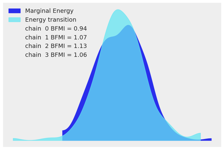
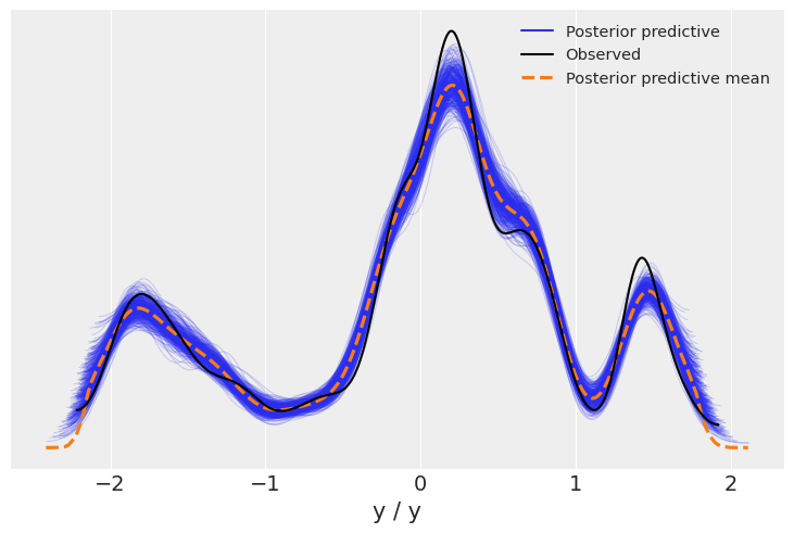
我们现在使用 arviz.plot_energy() 显示能量图，以直观检查模型的收敛性。然后，使用 arviz.plot_ppc()，我们将 后验预测样本 的分布与观测数据 \(\mathbf y\) 进行对比。该图提供了模型准确性的一般概念（注意，\(\mathbf y\) 的值实际上对应于 \(\mathbf y\) 的缩放版本）。

az.plot_energy(trace)
az.plot_ppc(trace);

后验可视化

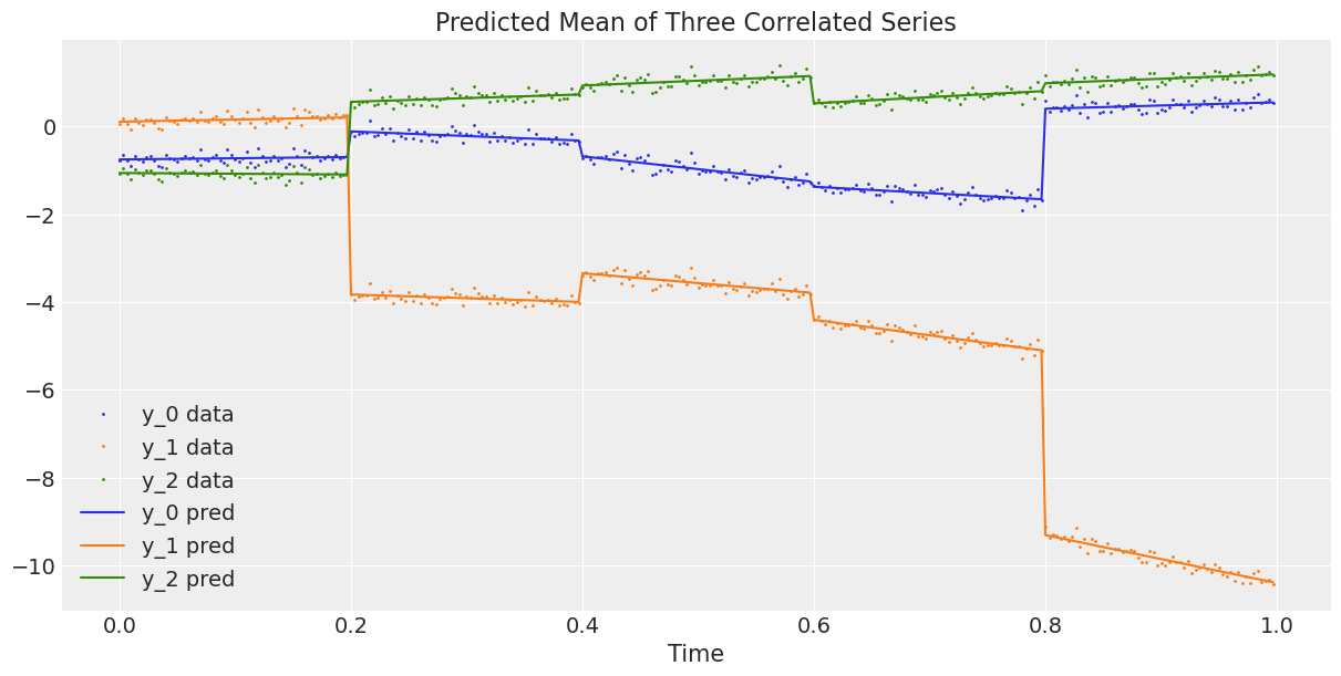
上面的图表看起来不错。现在我们将观察到的三维序列与平均预测的三维序列进行对比，或者换句话说，我们将数据与模型估计的回归曲线进行对比 （）。

# Compute the predicted mean of the multivariate GRWs
alpha_mean = trace.posterior["alpha"].mean(dim=("chain", "draw"))
beta_mean = trace.posterior["beta"].mean(dim=("chain", "draw"))

# Compute the predicted mean of the correlated series
y_pred = y_scaler.inverse_transform(
    alpha_mean[t_section].values + beta_mean[t_section].values * t_scaler.transform(t)
)

# Plot the predicted mean
fig, ax = plt.subplots(1, 1, figsize=(12, 6))
ax.plot(t, y, ".", markersize=2, label=("y_0 data", "y_1 data", "y_2 data"))
plt.gca().set_prop_cycle(None)
ax.plot(t, y_pred, label=("y_0 pred", "y_1 pred", "y_2 pred"))
ax.set_xlabel("Time")
ax.legend()
ax.set_title("Predicted Mean of Three Correlated Series");

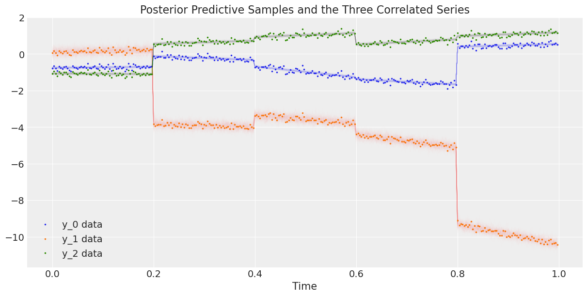
最后，我们将数据与后验预测样本进行绘制。

# Rescale the posterior predictive samples
ppc_y = y_scaler.inverse_transform(trace.posterior_predictive["y"].mean("chain"))

fig, ax = plt.subplots(1, 1, figsize=(12, 6))
# Plot the data
ax.plot(t, y, ".", markersize=3, label=("y_0 data", "y_1 data", "y_2 data"))
# Plot the posterior predictive samples
ax.plot(t, ppc_y.sel(y_="y_0").T, color="C0", alpha=0.003)
ax.plot(t, ppc_y.sel(y_="y_1").T, color="C1", alpha=0.003)
ax.plot(t, ppc_y.sel(y_="y_2").T, color="C2", alpha=0.003)
ax.set_xlabel("Time")
ax.legend()
ax.set_title("Posterior Predictive Samples and the Three Correlated Series");

作者

• 由 Lorenzon Itoniazzi 于 2021 年 10 月更新为最佳实践（pymc-examples#195）

• 由 Chris Fonnesbeck 于 2023 年 2 月更新至 v5

参考资料

[1]

丹尼尔·莱万多夫斯基、多罗塔·库罗维卡和哈里·乔。基于藤蔓和扩展洋葱方法生成随机相关矩阵。多元分析杂志，100(9):1989–2001, 2009.

水印

%load_ext watermark
%watermark -n -u -v -iv -w -p theano,xarray

Last updated: Thu Feb 02 2023

Python implementation: CPython
Python version       : 3.9.15
IPython version      : 8.7.0

theano: not installed
xarray: 2022.12.0

pytensor  : 2.8.11
numpy     : 1.23.5
pymc      : 5.0.1
sys       : 3.9.15 | packaged by conda-forge | (main, Nov 22 2022, 08:48:25) 
[Clang 14.0.6 ]
matplotlib: 3.6.2
arviz     : 0.14.0

Watermark: 2.3.1

许可证声明

本示例库中的所有笔记本均在MIT许可证下提供，该许可证允许修改和重新分发，前提是保留版权和许可证声明。

引用 PyMC 示例

要引用此笔记本，请使用Zenodo为pymc-examples仓库提供的DOI。

重要

许多笔记本是从其他来源改编的：博客、书籍……在这种情况下，您应该引用原始来源。

同时记得引用代码中使用的相关库。

这是一个BibTeX的引用模板：

@incollection{citekey,
  author    = "<notebook authors, see above>",
  title     = "<notebook title>",
  editor    = "PyMC Team",
  booktitle = "PyMC examples",
  doi       = "10.5281/zenodo.5654871"
}

渲染后可能看起来像：