从生成图导出的时间序列模型#

在本笔记本中，我们展示了如何从生成图开始建模和拟合时间序列模型。特别是，我们解释了如何使用scan在PyMC模型中高效地进行循环。

动机

为什么我们要这样做，而不是直接使用 AR？有什么好处？

PyMC 中预构建的时间序列模型非常有用且易于使用。然而，它们并不足够灵活，无法用于建模更复杂的时间序列模型。通过使用生成图，我们可以建模任何我们想要的时间序列模型，只要我们能够以生成图的形式定义它。例如：

具有不同噪声分布的自回归模型（例如 StudentT 噪声）。
指数平滑模型。
ARIMA-GARCH 模型。

对于这个例子，我们考虑一个自回归模型 AR(2)。回顾一下，AR(2) 模型定义为：

\[ \begin{align*} y_t &= \rho_1 y_{t-1} + \rho_2 y_{t-2} + \varepsilon_t, \quad \varepsilon_t \sim \mathcal{N}(0, \sigma^2) \end{align*} \]

也就是说，我们有一个关于时间序列前两个滞后的递归线性模型。

定义AR(2)过程#

我们首先将AR(2)模型的生成图编码为一个函数 ar_dist。策略是将此函数作为自定义分布通过 CustomDist 在 PyMC 模型中传递。

我们需要指定初始状态（ar_init）、自回归系数（rho）和噪声的标准差（sigma）。给定这些参数，我们可以使用scan操作定义AR(2)模型的生成图。

这些函数都是什么？

起初，看到所有这些函数可能会让人感到有些不知所措。然而，它们只是用于定义AR(2)模型生成图的辅助函数。

collect_default_updates() 告诉 PyMC 在生成图中的随机变量（RV）应该在循环的每次迭代中更新。如果我们不这样做，随机状态将不会在时间步之间更新，我们将一遍又一遍地采样相同的创新。
scan 是在 PyMC 模型内部进行循环的高效方法。它类似于 Python 中的 for 循环，但它是为 pytensor 优化的。我们需要指定以下参数：
- fn: 定义过渡陡度的函数。
- outputs_info: 这是描述递归计算输出初始状态的变量或字典列表。该字典的一个常见键是 taps，它指定要跟踪的前几个时间步。在这种情况下，我们跟踪最后两个时间步（滞后）。
- non_sequences: 传递给fn在每一步的参数列表。在这种情况下，是AR(2)模型的自回归系数和噪声标准差。
- n_steps: 循环的步数。
- strict: 如果True，fn中使用的所有共享变量必须作为non_sequences或sequences的一部分提供（在这个例子中，我们没有使用sequences参数，它是描述scan需要迭代的变量或字典的列表。在这种情况下，我们可以简单地遍历时间步长）。

让我们看看具体的实现：

lags = 2  # Number of lags
timeseries_length = 100  # Time series length


# This is the transition function for the AR(2) model.
# We take as inputs previous steps and then specify the autoregressive relationship.
# Finally, we add Gaussian noise to the model.
def ar_step(x_tm2, x_tm1, rho, sigma):
    mu = x_tm1 * rho[0] + x_tm2 * rho[1]
    x = mu + pm.Normal.dist(sigma=sigma)
    return x, collect_default_updates([x])


# Here we actually "loop" over the time series.
def ar_dist(ar_init, rho, sigma, size):
    ar_innov, _ = pytensor.scan(
        fn=ar_step,
        outputs_info=[{"initial": ar_init, "taps": range(-lags, 0)}],
        non_sequences=[rho, sigma],
        n_steps=timeseries_length - lags,
        strict=True,
    )

    return ar_innov

生成AR(2)图表#

现在我们已经实现了AR(2)步骤，我们可以为参数rho、sigma和初始状态ar_init分配先验。

coords = {
    "lags": range(-lags, 0),
    "steps": range(timeseries_length - lags),
    "timeseries_length": range(timeseries_length),
}
with pm.Model(coords=coords, check_bounds=False) as model:
    rho = pm.Normal(name="rho", mu=0, sigma=0.2, dims=("lags",))
    sigma = pm.HalfNormal(name="sigma", sigma=0.2)

    ar_init = pm.Normal(name="ar_init", sigma=0.5, dims=("lags",))

    ar_innov = pm.CustomDist(
        "ar_dist",
        ar_init,
        rho,
        sigma,
        dist=ar_dist,
        dims=("steps",),
    )

    ar = pm.Deterministic(
        name="ar", var=pt.concatenate([ar_init, ar_innov], axis=-1), dims=("timeseries_length",)
    )


pm.model_to_graphviz(model)

../_images/2fcb5b498136c7ab819bc3deae02d4241e402621fda765cd46c6a566b7baa44c.svg

先验#

让我们从先验分布中采样，看看AR(2)模型是如何表现的。

with model:
    prior = pm.sample_prior_predictive(samples=500, random_seed=rng)

Sampling: [ar_dist, ar_init, rho, sigma]

_, ax = plt.subplots()
for i, hdi_prob in enumerate((0.94, 0.64), 1):
    hdi = az.hdi(prior.prior["ar"], hdi_prob=hdi_prob)["ar"]
    lower = hdi.sel(hdi="lower")
    upper = hdi.sel(hdi="higher")
    ax.fill_between(
        x=np.arange(timeseries_length),
        y1=lower,
        y2=upper,
        alpha=(i - 0.2) * 0.2,
        color="C0",
        label=f"{hdi_prob:.0%} HDI",
    )
ax.plot(prior.prior["ar"].mean(("chain", "draw")), color="C0", label="Mean")
ax.legend(loc="upper right")
ax.set_xlabel("time")
ax.set_title("AR(2) Prior Samples", fontsize=18, fontweight="bold");

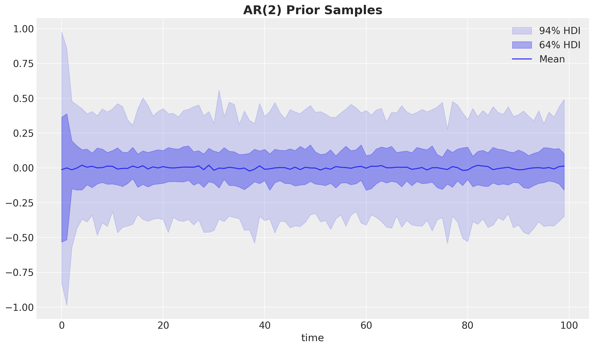
../_images/45f3badc36e8369f03ed13606f15c359042fcb3a28423d33856d1101e30a8ad4.png

鉴于我们对rho参数的先验分布是弱信息性的且以零为中心，先验分布在零附近是一个平稳过程，这并不令人惊讶。

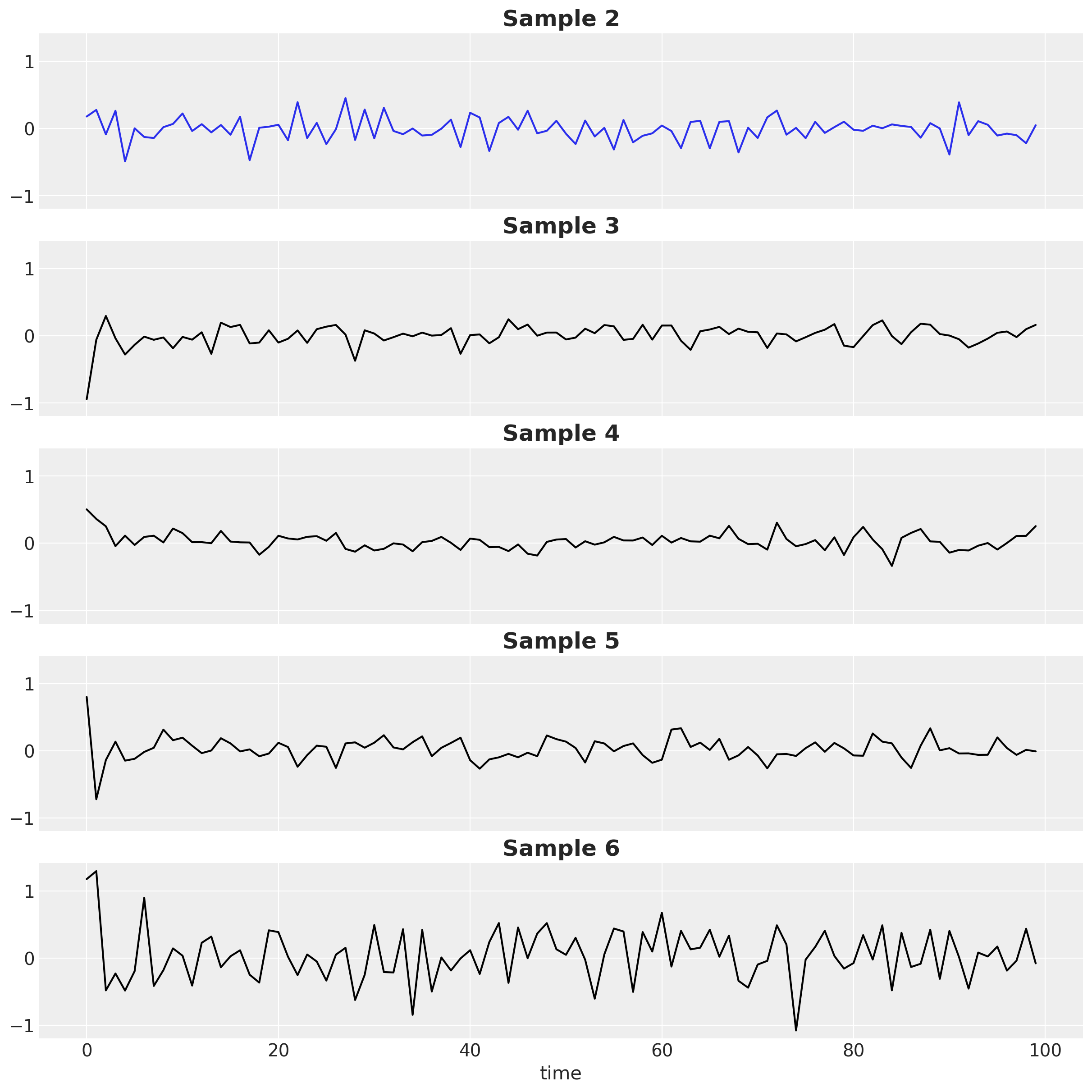
让我们查看单个样本，以感受生成序列的异质性：

fig, ax = plt.subplots(
    nrows=5, ncols=1, figsize=(12, 12), sharex=True, sharey=True, layout="constrained"
)
chosen_draw = 2

for i, axi in enumerate(ax, start=chosen_draw):
    axi.plot(
        prior.prior["ar"].isel(draw=i, chain=0),
        color="C0" if i == chosen_draw else "black",
    )
    axi.set_title(f"Sample {i}", fontsize=18, fontweight="bold")
ax[-1].set_xlabel("time");

../_images/a6263f09315e48c7a53e097c19217e14ed6cd680ff06753214d5a89c4ad5bd22.png

后验#

接下来，我们希望在AR(2)模型上基于一些观测数据进行条件处理，以便我们可以进行参数恢复分析。我们使用observe()操作。

# select a random draw from the prior
prior_draw = prior.prior.isel(chain=0, draw=chosen_draw)
test_data = prior_draw["ar_dist"].to_numpy()

with pm.observe(model, {"ar_dist": test_data}) as observed_model:
    trace = pm.sample(chains=4, random_seed=rng)

Auto-assigning NUTS sampler...
Initializing NUTS using jitter+adapt_diag...
Multiprocess sampling (4 chains in 4 jobs)
NUTS: [rho, sigma, ar_init]

Sampling 4 chains for 1_000 tune and 1_000 draw iterations (4_000 + 4_000 draws total) took 8 seconds.

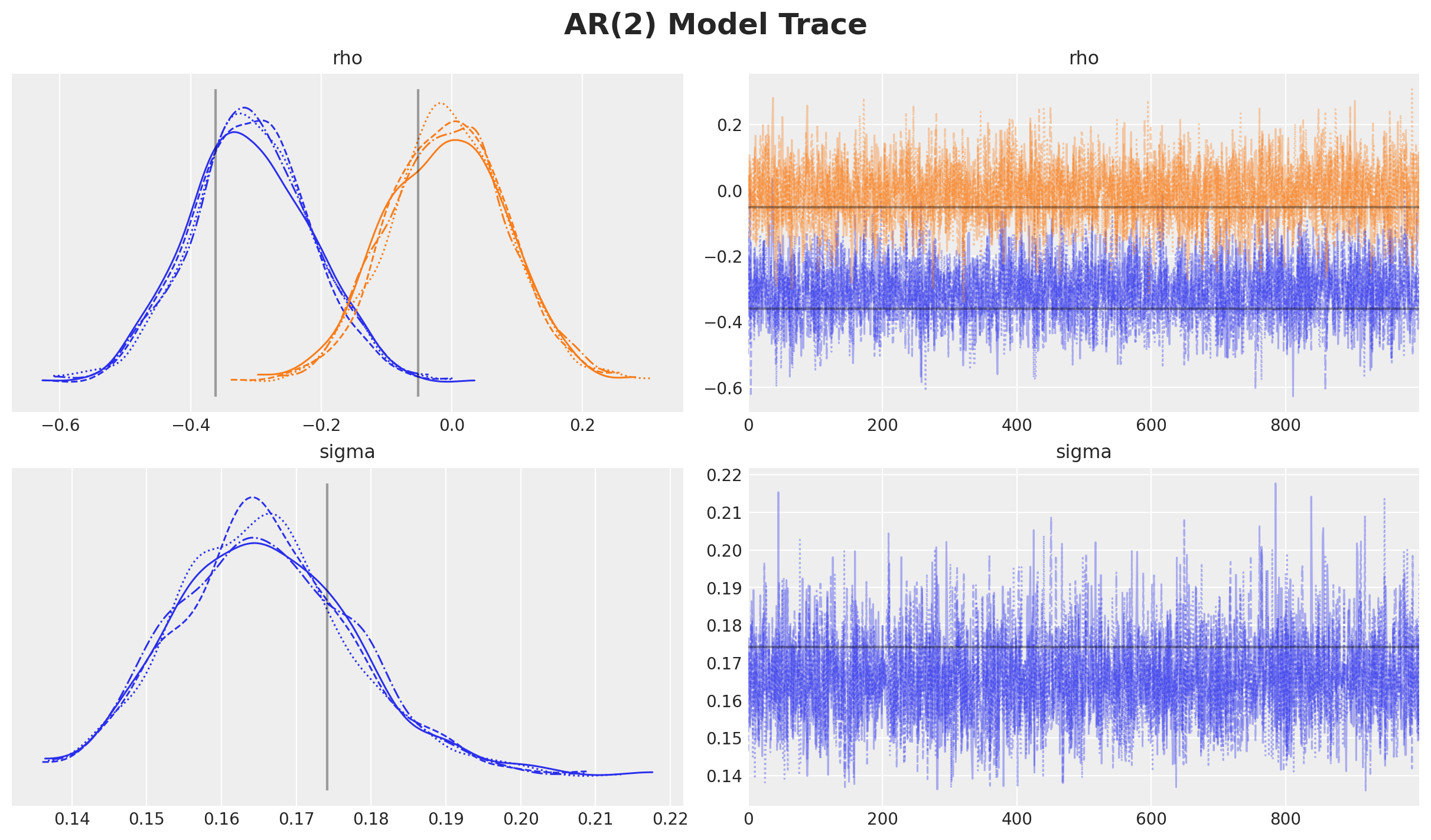
让我们绘制参数的轨迹和后验分布。

# Get the true values of the parameters from the prior draw
rho_true = prior_draw["rho"].to_numpy()
sigma_true = prior_draw["sigma"].to_numpy()
ar_obs = prior_draw["ar"].to_numpy()

axes = az.plot_trace(
    data=trace,
    var_names=["rho", "sigma"],
    compact=True,
    lines=[
        ("rho", {}, rho_true),
        ("sigma", {}, sigma_true),
    ],
    backend_kwargs={"figsize": (12, 7), "layout": "constrained"},
)
plt.gcf().suptitle("AR(2) Model Trace", fontsize=18, fontweight="bold");

../_images/f87a78ef0f724c8cc4618c870a2d7811d16c58595aa080a23c5dcdeb7d9a3bc9.png

axes = az.plot_posterior(
    trace, var_names=["rho", "sigma"], ref_val=[*rho_true, sigma_true], figsize=(15, 5)
)
plt.gcf().suptitle("AR(2) Model Parameters Posterior", fontsize=18, fontweight="bold");

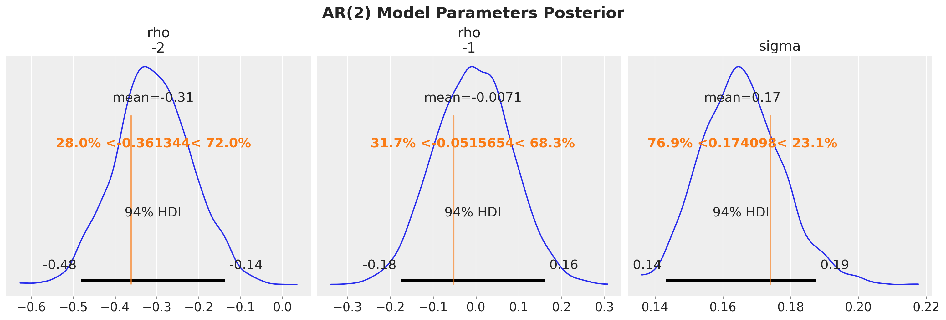
../_images/ccfaf92c6898bd2f63ec1081f30310187fc7778649da3d0496a780eecf44b0b6.png

我们看到我们已经成功恢复了模型的真实参数。

后验预测#

最后，我们可以使用后验样本从AR(2)模型生成新数据。然后，我们可以将生成的数据与观测数据进行比较，以检查模型的拟合优度。

with observed_model:
    post_pred = pm.sample_posterior_predictive(trace, random_seed=rng)

Sampling: [ar_dist]

post_pred_ar = post_pred.posterior_predictive["ar"]

_, ax = plt.subplots()
for i, hdi_prob in enumerate((0.94, 0.64), 1):
    hdi = az.hdi(post_pred_ar, hdi_prob=hdi_prob)["ar"]
    lower = hdi.sel(hdi="lower")
    upper = hdi.sel(hdi="higher")
    ax.fill_between(
        x=post_pred_ar["timeseries_length"],
        y1=lower,
        y2=upper,
        alpha=(i - 0.2) * 0.2,
        color="C0",
        label=f"{hdi_prob:.0%} HDI",
    )
ax.plot(
    post_pred_ar["timeseries_length"],
    post_pred_ar.mean(("chain", "draw")),
    color="C0",
    label="Mean",
)
ax.plot(ar_obs, color="black", label="Observed")
ax.legend(loc="upper right")
ax.set_xlabel("time")
ax.set_title("AR(2) Posterior Predictive Samples", fontsize=18, fontweight="bold");

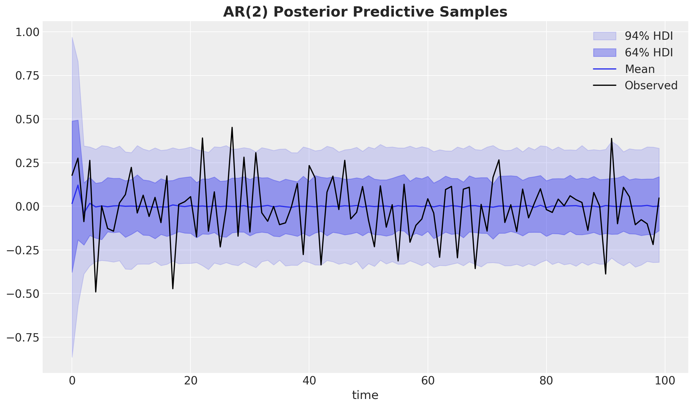
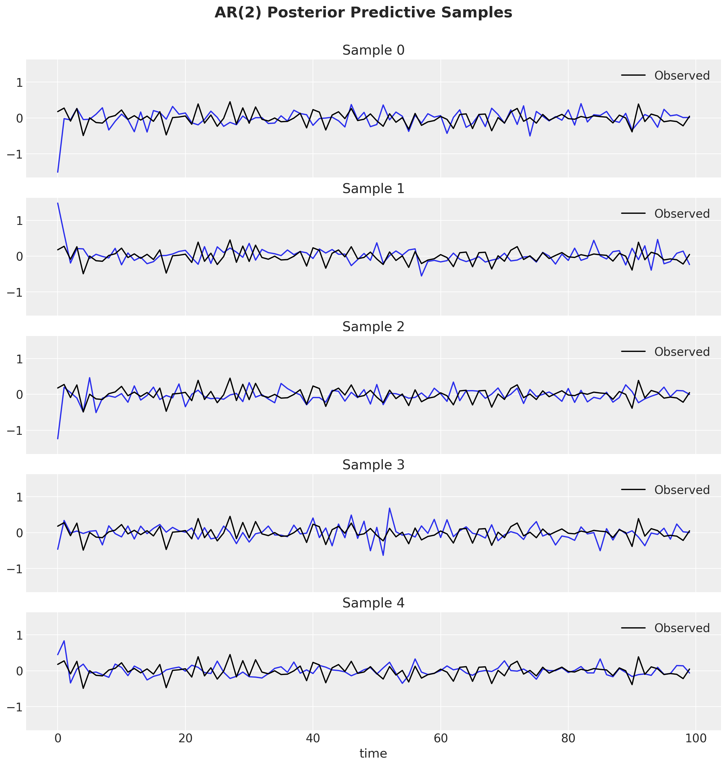
../_images/bbcee45009ab3e86bb315f431ef9f519501895eeaceab4c466d7a7510c399e7f.png

总体而言，我们看到模型正在捕捉时间序列的全局动态。为了更好地了解模型，我们可以绘制一部分后验样本并与观测数据进行比较。

fig, ax = plt.subplots(
    nrows=5, ncols=1, figsize=(12, 12), sharex=True, sharey=True, layout="constrained"
)
for i, axi in enumerate(ax):
    axi.plot(post_pred.posterior_predictive["ar"].isel(draw=i, chain=0), color="C0")
    axi.plot(ar_obs, color="black", label="Observed")
    axi.legend(loc="upper right")
    axi.set_title(f"Sample {i}")

ax[-1].set_xlabel("time")

fig.suptitle("AR(2) Posterior Predictive Samples", fontsize=18, fontweight="bold", y=1.05);

../_images/8c9be891a52dc79ac7dc6007638d0307a8b46b2bae58af516d68cc5ea41e0862.png

条件和无条件后验

许多用户会对这个后验感到惊讶，因为他们习惯于看到条件一步预测，即

\[ P(x_{t} \: | \: \{ x_{\tau} \}_{\tau = 1} ^{t - 1}) \]

（在 statsmodels/stata/everything 中得到的结果），这些结果更加紧密，并且更贴近数据。

让我们看看如何在 PyMC 中实现这一点！关键的观察是，我们需要将观测数据显式地传递到生成图中的“for 循环”中。也就是说，我们需要将其传递到 scan 函数中。

def conditional_ar_dist(y_data, rho, sigma, size):
    # Here we condition on the observed data by passing it through the `sequences` argument.
    ar_innov, _ = pytensor.scan(
        fn=ar_step,
        sequences=[{"input": y_data, "taps": list(range(-lags, 0))}],
        non_sequences=[rho, sigma],
        n_steps=timeseries_length - lags,
        strict=True,
    )

    return ar_innov

然后我们可以简单地从后验预测分布中生成样本。请注意，我们需要“重写”生成图以包括条件转移步骤。当你调用sample_posterior_predictive()时，PyMC将尝试将活动模型上下文中的随机变量名称与提供的idata.posterior中的名称匹配。如果找到匹配项，则将忽略指定的模型先验，并替换为从后验中抽取的样本。这意味着我们可以将任何先验放在这些参数上，因为它将被忽略。我们选择Flat，因为你无法从中采样。这样，如果PyMC没有找到我们某个先验的匹配项，我们将得到一个错误，让我们知道某些地方不对劲。有关这种跨模型预测的详细解释，请参阅这篇精彩的博文使用PyMC进行模型外预测。

警告

我们需要将坐标 steps 向前移动一步！原因是（例如）step=1 的数据用于创建 step=2 的预测。如果不进行移动，step=0 的预测将被错误地标记为 step=0，并且模型看起来会比实际情况更好。

coords = {
    "lags": range(-lags, 0),
    "steps": range(-1, timeseries_length - lags - 1),  # <- Coordinate shift!
    "timeseries_length": range(1, timeseries_length + 1),  # <- Coordinate shift!
}
with pm.Model(coords=coords, check_bounds=False) as conditional_model:
    y_data = pm.Data("y_data", ar_obs)
    rho = pm.Flat(name="rho", dims=("lags",))
    sigma = pm.Flat(name="sigma")

    ar_innov = pm.CustomDist(
        "ar_dist",
        y_data,
        rho,
        sigma,
        dist=conditional_ar_dist,
        dims=("steps",),
    )

    ar = pm.Deterministic(
        name="ar", var=pt.concatenate([ar_init, ar_innov], axis=-1), dims=("timeseries_length",)
    )

    post_pred_conditional = pm.sample_posterior_predictive(trace, var_names=["ar"], random_seed=rng)

Sampling: [ar_dist]

让我们可视化条件后验预测分布，并将其与statsmodels结果进行比较：

# PyMC conditional posterior predictive samples
conditional_post_pred_ar = post_pred_conditional.posterior_predictive["ar"]

# Statsmodels AR(2) model
mod = sm.tsa.ARIMA(ar_obs, order=(2, 0, 0))
res = mod.fit()

_, ax = plt.subplots()
for i, hdi_prob in enumerate((0.94, 0.64), 1):
    hdi = az.hdi(conditional_post_pred_ar, hdi_prob=hdi_prob)["ar"]
    lower = hdi.sel(hdi="lower")
    upper = hdi.sel(hdi="higher")
    ax.fill_between(
        x=conditional_post_pred_ar["timeseries_length"],
        y1=lower,
        y2=upper,
        alpha=(i - 0.2) * 0.2,
        color="C1",
        label=f"{hdi_prob:.0%} HDI",
    )
ax.plot(
    conditional_post_pred_ar["timeseries_length"],
    conditional_post_pred_ar.mean(("chain", "draw")),
    color="C1",
    label="Mean",
)
ax.plot(ar_obs, color="black", label="Observed")
ax.plot(
    conditional_post_pred_ar["timeseries_length"],
    res.fittedvalues,
    color="C2",
    label="statsmodels",
)
ax.legend(loc="lower center", bbox_to_anchor=(0.5, -0.2), ncol=5)
ax.set_xlabel("time")
ax.set_title("AR(2) Conditional Posterior Predictive Samples", fontsize=18, fontweight="bold");

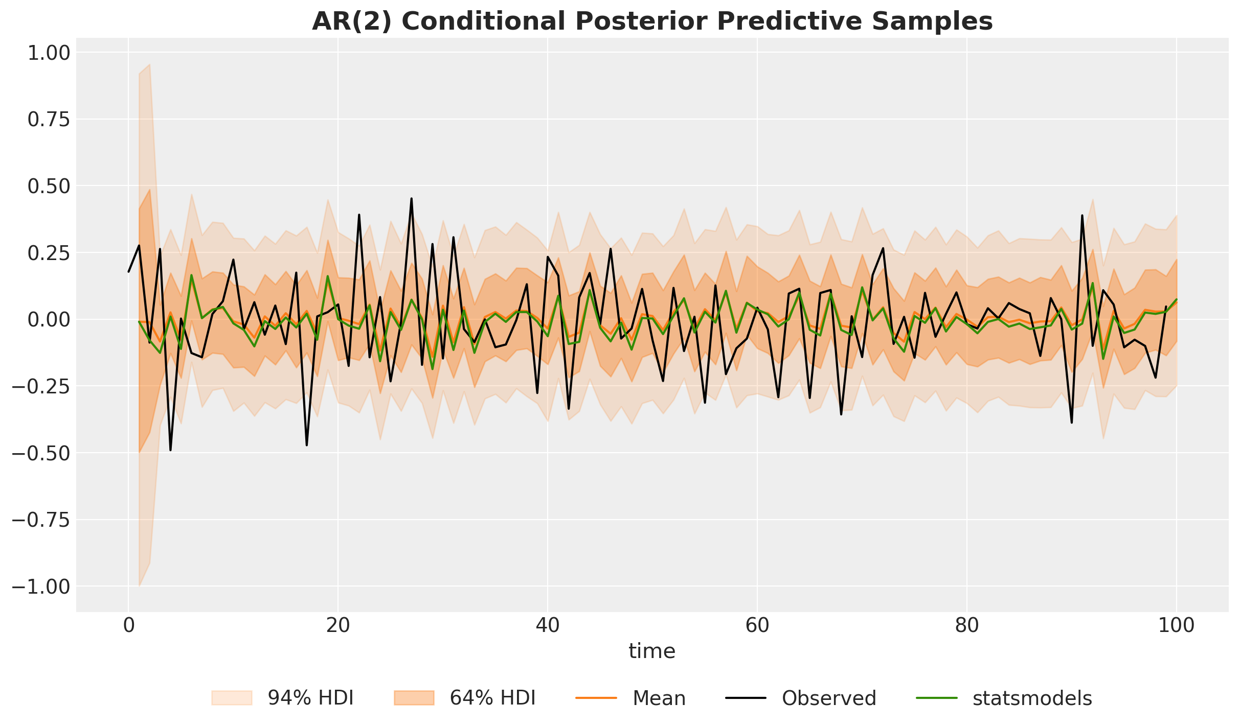
../_images/52c39b2e97255cfe8826fc107d6cbe007815468dda4851bbadd96d1064abda55.png

我们确实看到这些可信区间比无条件的更紧。

以下是一些额外的备注：

没有对 \(y_0\) 的预测，因为我们没有观察到 \(y_{t - 1}\)。
预测似乎在“追逐”数据，因为这正是我们在做的。在每一步，我们重置为观测数据并进行一次预测。

注意

相对于statsmodels参考，我们在初始化上略有不同。这是有道理的，因为他们使用了一些复杂的MLE初始化技巧，而我们将其估计为一个参数。这种差异应该在我们迭代序列时消失，而我们确实看到它确实如此。

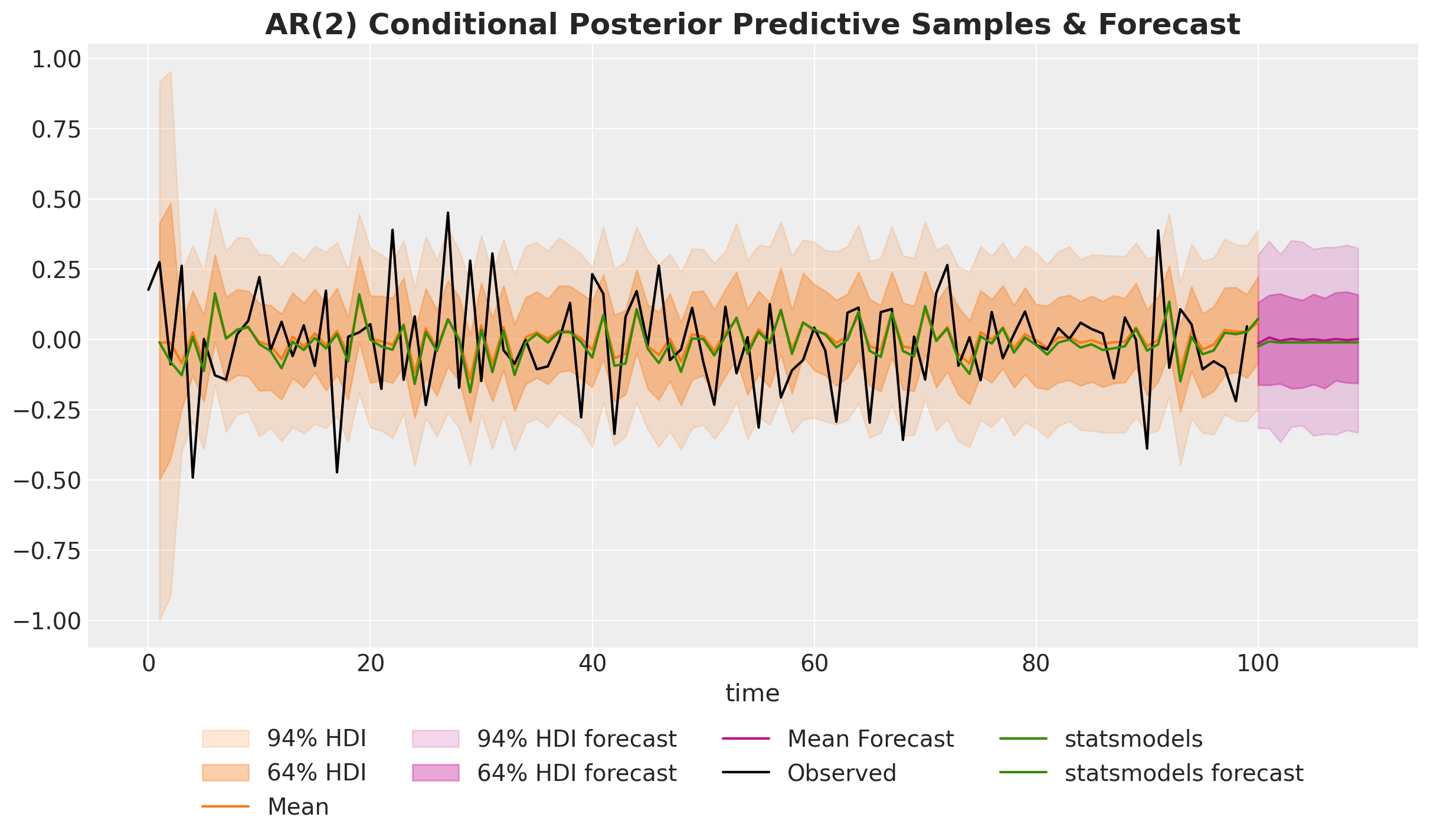
样本外预测#

在最后这一节中，我们描述如何生成样本外预测。

# Specify the number of steps to forecast
forecast_steps = 10

这个想法是使用后验样本和最新的两个数据点（因为我们有一个AR(2)模型）来生成预测：

coords = {
    "lags": range(-lags, 0),
    "steps": range(timeseries_length, timeseries_length + forecast_steps),
}
with pm.Model(coords=coords, check_bounds=False) as forecasting_model:
    forecast_initial_state = pm.Data("forecast_initial_state", ar_obs[-lags:], dims=("lags",))
    rho = pm.Flat(name="rho", dims=("lags",))
    sigma = pm.Flat(name="sigma")

    def ar_dist_forecasting(forecast_initial_state, rho, sigma, size):
        ar_innov, _ = pytensor.scan(
            fn=ar_step,
            outputs_info=[{"initial": forecast_initial_state, "taps": range(-lags, 0)}],
            non_sequences=[rho, sigma],
            n_steps=forecast_steps,
            strict=True,
        )
        return ar_innov

    ar_innov = pm.CustomDist(
        "ar_dist",
        forecast_initial_state,
        rho,
        sigma,
        dist=ar_dist_forecasting,
        dims=("steps",),
    )

    post_pred_forecast = pm.sample_posterior_predictive(
        trace, var_names=["ar_dist"], random_seed=rng
    )

Sampling: [ar_dist]

我们可以可视化样本外的预测结果，并将其与statsmodels的结果进行比较。

forecast_post_pred_ar = post_pred_forecast.posterior_predictive["ar_dist"]

_, ax = plt.subplots()
for i, hdi_prob in enumerate((0.94, 0.64), 1):
    hdi = az.hdi(conditional_post_pred_ar, hdi_prob=hdi_prob)["ar"]
    lower = hdi.sel(hdi="lower")
    upper = hdi.sel(hdi="higher")
    ax.fill_between(
        x=conditional_post_pred_ar["timeseries_length"],
        y1=lower,
        y2=upper,
        alpha=(i - 0.2) * 0.2,
        color="C1",
        label=f"{hdi_prob:.0%} HDI",
    )

ax.plot(
    conditional_post_pred_ar["timeseries_length"],
    conditional_post_pred_ar.mean(("chain", "draw")),
    color="C1",
    label="Mean",
)

for i, hdi_prob in enumerate((0.94, 0.64), 1):
    hdi = az.hdi(forecast_post_pred_ar, hdi_prob=hdi_prob)["ar_dist"]
    lower = hdi.sel(hdi="lower")
    upper = hdi.sel(hdi="higher")
    ax.fill_between(
        x=forecast_post_pred_ar["steps"],
        y1=lower,
        y2=upper,
        alpha=(i - 0.2) * 0.2,
        color="C3",
        label=f"{hdi_prob:.0%} HDI forecast",
    )

ax.plot(
    forecast_post_pred_ar["steps"],
    forecast_post_pred_ar.mean(("chain", "draw")),
    color="C3",
    label="Mean Forecast",
)


ax.plot(ar_obs, color="black", label="Observed")
ax.plot(
    conditional_post_pred_ar["timeseries_length"],
    res.fittedvalues,
    color="C2",
    label="statsmodels",
)
ax.plot(
    forecast_post_pred_ar["steps"],
    res.forecast(forecast_steps),
    color="C2",
    label="statsmodels forecast",
)
ax.legend(loc="upper center", bbox_to_anchor=(0.5, -0.1), ncol=4)
ax.set_xlabel("time")
ax.set_title(
    "AR(2) Conditional Posterior Predictive Samples & Forecast",
    fontsize=18,
    fontweight="bold",
);

../_images/291bb5c10dcdd2c83daa2c3e3988342d7bceeaedac92065c57046f3ec1ce0d67.png

作者#

由 Jesse Grabowski、Juan Orduz 和 Ricardo Vieira 于2024年3月撰写

水印#

%load_ext watermark
%watermark -n -u -v -iv -w -p pytensor

Last updated: Sun Jul 28 2024

Python implementation: CPython
Python version       : 3.12.4
IPython version      : 8.25.0

pytensor: 2.23.0

matplotlib : 3.8.4
numpy      : 1.26.4
pytensor   : 2.23.0
statsmodels: 0.14.2
arviz      : 0.17.1
pymc       : 5.16.1

Watermark: 2.4.3

许可证声明#

本示例库中的所有笔记本均在MIT许可证下提供，该许可证允许修改和重新分发，前提是保留版权和许可证声明。

引用 PyMC 示例#

要引用此笔记本，请使用Zenodo为pymc-examples仓库提供的DOI。

重要

许多笔记本是从其他来源改编的：博客、书籍……在这种情况下，您应该引用原始来源。

同时记得引用代码中使用的相关库。

这是一个BibTeX的引用模板：

@incollection{citekey,
  author    = "<notebook authors, see above>",
  title     = "<notebook title>",
  editor    = "PyMC Team",
  booktitle = "PyMC examples",
  doi       = "10.5281/zenodo.5654871"
}

渲染后可能看起来像：

分类

标签